A Bird’s Eye View of Linear Algebra: Systems of Equations, Linear Regression, and Neural Networks

The humble matrix multiplication along with its inverse is almost exclusively what’s going on in many simple ML models

This is the fourth chapter of the in-progress book on linear algebra, “A birds eye view of linear algebra”. The table of contents so far:

Chapter-1: The basics
Chapter-2: The measure of a map — determinants
Chapter-3: Why is matrix multiplication the way it is?
Chapter-4 (current): Systems of equations, linear regression and neural networks

All images in this blog, unless otherwise stated, are by the author.

I) Introduction

Modern AI models leverage high dimensional vector spaces to encode information. And the tool we have for reasoning about high dimensional spaces and mappings between them is linear algebra.

And within that field, matrix multiplication (along with its inverse) is literally all you need to build many simple machine learning models end to end. Which is why spending the time to understand it really well is a great investment. And this is what we did in chapter 3.

These simple models, useful in their own right, form the building blocks of more complex ML and AI models with state of the art performance.

We’ll cover a few of these applications (from linear regression to elementary neural networks) in this chapter.

But first, we need to go to the simplest case in the simplest model — when the number of data points equals the number of model parameters. The case of solving a system of linear equations.

II) Systems of linear equations

We have finally arrived (in the context of this book) at the heart of linear algebra. Solving systems of linear equations is how we discovered linear algebra in the first place and the motivations for most concepts in this field have deep roots in this application.

Let’s start simple and one dimensional. The concept of division is rooted in one dimensional linear equations.

ax = b

The equation reads, “what number when multiplied by a leads to b”. And the solution is what defines scalar division:

x = b/a _(1)

This is with one dimension, x. Most interesting things happen when things go multi-dimensional. So instead of just one variable, x, we have n variables (x_1, x_2, x_3, …, x_n).

And as soon as you go multi-dimensional, linear algebra jumps into the scene.

When things get multi-dimensional, linear algebra makes an entry. Image by midjourney.

Now, instead of a.x = b, our equation should include the n variables, x_1, x_2, x_3, …, x_n. And just like x had the coefficient, a, before; each of the x_i’s gets its own coefficient, a_i this time.

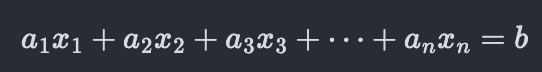
But unlike in the one dimensional case, this one equation is not enough to solve for the x’s since it doesn’t uniquely specify them. For example, we can pick any values we want for x_2, x_3,…, x_n (ex: all 0’s) and only then will we have a unique value for x_1. If we already knew the values of x_1, x_2, …, x_n and wanted to communicate them in the form of a system of equations, they would look something like:

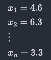
So, we needed n equations (equal to the number of variables). Any general system can now be created by “mixing” the equations above by taking linear combinations of them. This allows adding any two equations and multiplying any of the equations by any scalar. These operations will obviously not change the solution of the system (or the question of its existence).

For example, we can add three times the second equation to the first equation and get:

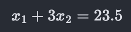
Then we can replace the first equation (x_1=4.6) by this one and the resulting system will still have the same solution (because we can just undo the change we made by subtracting three times the second equation from the new first equation). If we “mix” in this way very throughly, replacing one of the equations at random with the “mixed” one and repeat many times, we’ll end up with n equations each of which involves multiples of all the n variables.

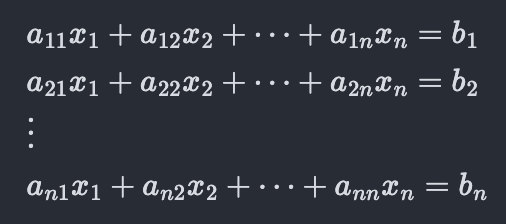
The coefficients a_{ij} look an awfully lot like the elements of a square matrix. And indeed, from what we learnt about matrix vector multiplication in chapter 3 (see animation-1 in section III-A), we can express the system of equations as:

Eq (1) Matrix form of the system of linear equations.

And just like in equation (1) we took the multiplicative inverse to get the scalar variable, x (x=b/a), here we take the inverse of matrix multiplication to get the vector, x.

And we have reached the iconic equation where it all started. Where linear algebra began. The system of linear equations. There is a whole science behind calculating the inverse and doing it well which we will cover in subsequent chapters.

Note that the number of rows in the A matrix was the number of equations in the system and the number of columns was the number of variables.

Geometrically, each equation is a hyperplane in the space with one lower dimensionality. Take the system of equations below:

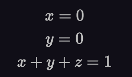
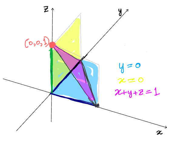
The solution to this system of equations is (x=0, y=0, z=1). Since there are three variables in this system (x, y and z), the vector space is three dimensional as shown in figure-1 below. Refer to that figure for the proceeding discussion.

The x=0 equation corresponds to the yellow hyper-plane in this 3-d space. Since the equation represents the addition of one constraint, the dimensionality of the space where this equation is satisfied goes down by one (3–1=2). Similarly, the y=0 equation corresponds to the blue hyperplane, also two dimensional. Now that we have two equations, so two constraints. The dimensionality of the sub-space where both of them are satisfied will go down by two, making it 3–2=1 dimensional. A one dimensional sub-space is just a line, and indeed we get the green line figure-1. Finally, when we add the third equation, x+y+z=1, represented by the pink plane. We now have three equations/ constraints. And they restrict the dimensionality of the 3-d space by 3. So we’re left with 3–3 = 0 dimensions (which is a point) and indeed, we get the red point, the only element of the vector space that satisfies all three of the equations in the system simultaneously.

Figure-1: A system of equations in 3 variables. The space is three dimensional. Each equation carves out a hyper-plane one dimension lower. Combinations of two equations remove two dimensions and so on. Image by author.

In the example above, we had n equations and n variables. In general, they needn’t be the same. Let’s say there are n equations and m variables. It's clear from the figure above:

When n<m, we have more variables than equations and the system has no solution.
When n>m, we’ll have more equations than variables. There are now too many constraints to satisfy and we won’t be able to find any points in the vector space that satisfy all of them.
So when n=m, we should always have a single, unique solution? Not quite, there are ways things can go wrong (for all three cases).

II-A) How things go wrong

Consistency

One thing that will make any system have no solution is inconsistency. Say the first equation is 2x+y=3 and the second one is 2x+y = 5. Now, regardless of how many more equations we add, there will be no way to satisfy both of them simultaneously (they simply contradict each other). Any system that has those two equations is inconsistent.

Dependency

Next, the system could deceive us, looking like it has more equations than it actually does. The most obvious way this could happen is if we simply copy one of the equations. This will add one equation to the system, making it so that technically, we have m+1 equations now. It’s clear, however, that we didn’t really add any new information. The new equation we added is redundant. This is called a dependent system because some of our equations don’t bring any new information of their own but “depend” on others. If we downright plagiarize one of the equations, its going to be obvious to spot. But the same thing can be done in a more clandestine way. Instead of downright copying one of the equations, we can take a linear combination of a few of them to create a new one. The linear combination can be done in a way that it is almost impossible to spot just by looking at the equations that there is an “imposter equation” in the mix. Of course, once such a dependent equation is added into the mix, it is impossible to tell which one the “imposter” is, like the three spider men below.

Two Bob’s. But there can be only one. One of them is an imposter. Hard to tell which one. Much like dependent equations introduced in a linear system by taking linear combinations of the others. Image by midjourney.

The two problems of consistency and dependency manifest in the same way as far as the A matrix (from equation (1)) goes. The vector b then determines whether the system is inconsistent (no solution) or dependent (infinitely many solutions). What happens is that some of the rows of A turn out to be linear combinations of the others.

II-B) The case of data analysis

The case that is most interesting to us is building models on top of data. If you have data points collected independently, with an underlying random process (like data collection should be), it's almost certain that the rows of your data matrix won’t be linearly dependent (in probability terms, “almost surely”). So, we don’t have to worry about getting either an inconsistent or dependent system.

Also, we typically have many more rows (data points) than columns (variables/ features). So, the matrix will be “skinny”, with n>m.

A tall, skinny rectangular matrix of data with more rows than columns. Image by midjourney.

We’re firmly in the domain of no solution to the system of equations. If we choose any m of the n equations and delete/ ignore the rest, then we will be back to the m=m case with an equal number of equations and variables and now there will be a unique solution.

So, there are a total of (n choose m) points the hyperplanes corresponding to the equations in the system form. None of these points will lie on all the hyperplanes simultaneously.

Even though there is no point that simultaneously satisfies all the equations, we can still ask “what is the point in the entire vector space that comes closest to satisfying all the equations”. And this is where linear regression comes in.

II) Linear regression

Linear regression draws a linear hyperplane that is closest to the points in your data. Much like the ninja attempts to swing his sword in a way that its closest to as many leaves as possible. Image by midjourney.

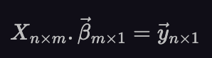
First, in the context of linear regression, the matrices and vectors are named slightly differently than they are with systems of equations. Now, the matrix of coefficients, A becomes the matrix that contains the data and we call it X. Each row of this matrix, the row vector x_i, is one data entry. The vector x contained the unknown variables in equation (1). Now, the unknown variables are the linear regression coefficients and we denote them, 𝛽. And finally, the right hand vector of the linear system, b becomes the vector that contains the dependent variable and we call it y. So, equation (1) in the context of linear regression becomes:

Eq (2): The basic equation of linear regression. Image by author.

Expanded out, this equation looks like the following:

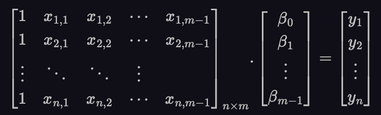
Notice the first column of 1’s. This corresponds to the constant term. For example, in the one variable case, without that column our model would be: y = m.x. This would exclude lines like y=x+1 from consideration. In order to consider lines like: y = mx+c (which we do want in most cases), we need that column of 1’s.

Just as with the linear system of equations, we’d like to take the multiplicative inverse of X on both sides and find 𝛽. Like this:

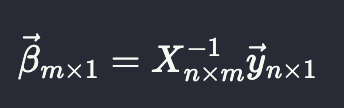
This equation doesn’t make any sense. The matrix, X is rectangular, so it can’t be inverted.

Unfortunately, this doesn’t make sense. Only square matrices can be inverted. Rectangular ones simply can’t. And our data matrix, X is rectangular with the number of rows (n) > number of columns (m).

One way to see this is that it represents a linear system with more equations than variables and the arguments of section II apply. In terms of the linear map behind the matrix, for a “skinny” rectangular matrix with more rows than columns (like X is), it won’t be a one to one mapping (multiple points from the same space will map to the same point in the second one, which isn’t allowed).

Is there a “hack” we can do to just make the matrix multiplied by 𝛽 a square one? The matrix, X is currently n⨉m. What if we multiplied by some other m⨉n matrix, U. Then, the resulting matrix, V will be square m⨉m.

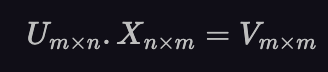
Pre-multiplying equation (2) by U, we are then able to invert the resulting matrix and get 𝛽.

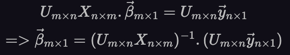
Now, the question is, where do we get this U matrix (m⨉n) from? The X matrix, n⨉m is what we have (the data itself). One thing we can do is flip the X matrix so its rows become its columns and columns become rows. This kind of operation on a matrix is called transpose, denoted by X^T visualized below.

Transpose of a matrix. Image credit: Wikipedia article on transpose.

So, we can replace U by the transpose of X. This leads to:

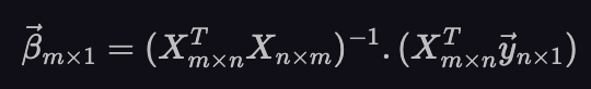
Eq (3): The linear regression coefficients.

And we have now found the coefficients of the regression model. If we get a new data point, x_new (in the form of a row vector) we can take its dot product with 𝛽 and obtain the corresponding y.

Where 𝛽 is given by equation (3) above. Now, we provided the motivation for replacing U by X^T since it was an obvious choice with the dimensions we were looking for. But, the same formula has a much stronger mathematical motivation.

II-A) Mathematical motivation

We need to motivate a specific value of 𝛽 (the one in equation (3)). So, let’s think about what happens for various values of 𝛽. As explained in animation-1, section III-A of chapter 3 (matrix multiplication), we can interpret X𝛽 as taking apart the column vectors of X and combining them into a single column vector via a linear combination. More specifically, we multiply the first column vector of X by the first element of the vector 𝛽, the second column vector by the second element and so on and then adding up all the results. So, as we change the vector 𝛽, we’re exploring the “column space” of the matrix X, which is the set of all vectors we can get via a linear combination of the column vectors of X. And then we also have the vector y, the right hand side of our equation (2). Just like the column vectors of X, the dimensionality of this vector is also n (the number of data points/ rows in the matrix).

The dimensionality of this vector space (that contains y and the column vectors of X) is n. On the other hand, the number of column vectors from X is m. And remember, we’re in the case where n>>m. So, the column space of X (space spanned by these m vectors) will have dimensionality m. This is much lower than n, the larger space where those column vectors live.

The vector y lives in the same larger space of dimensionality, n. Since the number of column vectors, m is so much smaller than n, the vector y will not be in the column space spanned by the column vectors of X, almost surely.

If it were, we’d have a 𝛽 that satisfies all the equations exactly. This is impossible to do (as discussed before). But, we still want to find a 𝛽 that brings it as close as possible to the vector, y. To do this, we minimize the distance between y and X𝛽.

Let’s take a concrete example. Say we have a data set with n=3 data points. In our regression model, we choose m=2 features. The X𝛽=y equation looks like this:

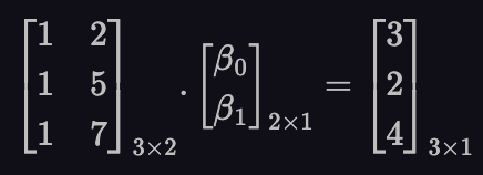
So, the matrix X has two column vectors, [1,1,1] and [2,5,7]. They live in a 3 dimensional space (n=3). These two column vectors are plotted in blue in figure-2 below. The space spanned by those vectors (column space) is two dimensional (m=2) and a section of it is shaded in pink.

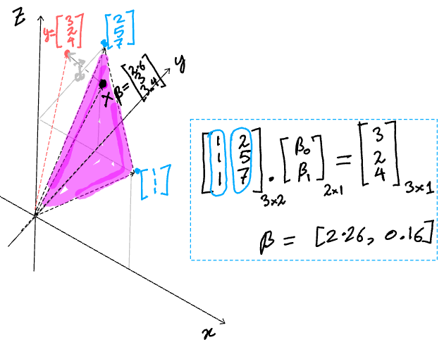
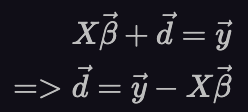
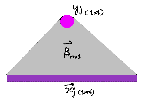
Figure-2: Demonstrating linear regression as an exploration of the column space of the data matrix, X. Image by author.

Now, look at the triangle formed by the black vector, grey vector and red vector. The black vector is X𝛽, the red vector is y and the grey vector is d. The three form a triangle and hence satisfy:

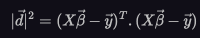
It’s this d vector whose length we want to find the point in the column space of X (controlled by 𝛽) that is closest to y.

We get the squared length of a column vector by matrix-multiplying its transpose with itself.

Finally, let’s take the derivative with respect to 𝛽 and set it to 0. This will give us the 𝛽 that minimized the squared length of vector d.

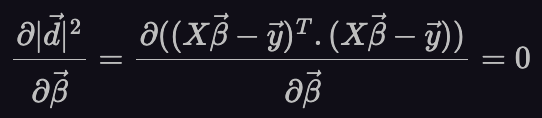
Here, we use equation (78) from the matrix cook-book, [2]. This leads to:

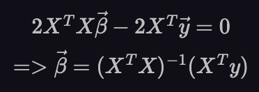
And this is the same as equation (3).

We motivated here with the column space of X (as explained in more detail in [1]). The same equations can also be motivated as minimizing the square error terms in the predicted and actual values of vector, y. This approach is covered in [2].

II-B) Online linear regression

Online linear regression. Data comes in as a constant stream, day over day. We need to keep our linear regression model up to date as that happens. Image by midjourney.

So far, we thought of linear regression as a static model where the data matrix, X and the corresponding vector of responses, y are given to us. Very often, we have data coming in as a constant stream over time. Some data points might drop today, some more tomorrow and so on. And we’d like our model to use a rolling window of data (say 30 days) and the parameters should be updated every day for the data from the last 30 days. The obvious way to do it is to use equation (3) on the past 30 days of data every day and refresh the parameters on a daily basis. But what if the number of data points, n (rows in the matrix X) is very large? That’ll make the computation in equation (3) very expensive. And if you think about the model yesterday versus today. Most of the data considered by the two models is the same because of the rolling window. On day 31, we used the data from day 1 to day 30 and on day 32, we used the data from day 2 to day 31. The data from day 2 to day 30 is common. What makes the model for day 32 different from the one on day 31 is that it does not consider all the data points that dropped on day 1 and does consider the ones that dropped on day 31. Apart from that, the vast majority of the data (days 2 through 29) is common. It seems wasteful then to ignore this and train the entire model from scratch everyday. If we could reformulate equation (3) in a way that its a sum over some function of the rows of X, x_i, we could keep adding in the contributions of new data as it came in while subtracting the contribution from the old data that falls out of the rolling window.

And one of the many interpretations of matrix multiplication we covered in chapter 3 helps us do just that. In section III-B of chapter 3 (around animation 5) the interpretation of matrix multiplication as a sum of outer products of the rows of the two matrices is covered. Using that, we can square the matrix on the left of equation (3) as:

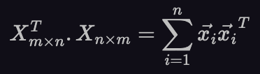
Here, the vector x_i is the i-th row of the matrix X. It has one row and m columns (1⨉m).

Similarly, the vector on the left side of that equation can be written as:

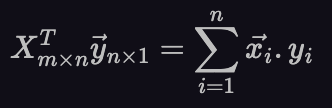
Since both the terms have been expressed as sums over the n data points, we can add and remove the contributions from individual data points at will. We can keep running versions of the matrix in equation (4) and vector in equation (5) based on the data points that fall in the last 7 days. If a data point falls outside the 30 day window, we can subtract the terms it corresponds to from both the equations and if a new data point comes in, we can add its terms to both the equations. And since m is small, we can efficiently calculate 𝛽, keeping it up to date every time we update those terms. This method can also be used to add weights to the data points. This can be useful if (for example), you’re getting data from multiple sources and want to weigh some of them more than others. You’d just multiply the weight, w_i for the i-th data point into each of the terms of equations (4) and (5).

III) Neural networks

Neural network architectures consist of layers of vectors. The first layer is the input layer, the last layer is the output layer and everything in between is a hidden layer. Image by midjourney.

Neural networks are machine learning models that are inspired by the neural connections in biological brains. They are the current weapon of choice in our quest towards artificial general intelligence. All recent advances, from text to image to conversation bots use models that are neural networks at their core.

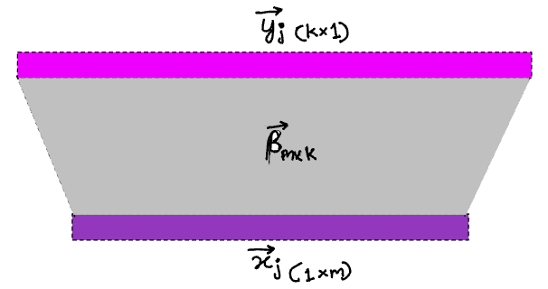
Linear regression can be thought of as the simplest possible neural network. Let’s concern ourselves with inference for now, the process of obtaining the output vector given an instance of the input to the model. For linear regression, we’ll get a row vector, x as input and a single scalar value, y as output. The parameter vector, 𝛽 takes us from the input to the output.

In linear regression, we get a vector corresponding to a new data point, x_j. This is multiplied with the parameter vector, beta to produce the response, y_j which is a single scalar. Image by author.

To extend this to neural networks, we generalize in two ways.

First, in order for the model to be able to output all kinds of interesting things like images, sentences, videos and spaceships, we need it to output not just a scalar (like with linear regression), but a vector. If this vector is high dimensional enough, any complex response we expect can be embedded effectively in its corresponding vector space.

So we need to go from vector->scalar for the case of linear regression to vector->vector. The scalar output is then just a special case, since its a one dimensional vector. This changes the picture above to this:

In general, we’d like the response, y to be a vector instead of a scalar. That way, we can embed complex information about the real world in that vector space. Image by author.

Now, the parameter vector, 𝛽 from before will need to become a parameter matrix. This is a linear map that maps the input vector to the output vector.

But, most interesting relationships in the real world are non-linear. To accommodate this, we first insert a bunch of intermediate “hidden layers”, shown in blue below.

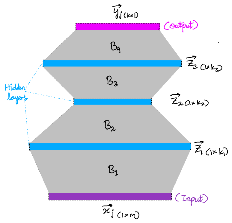
Architecture of a deep neural network. The hidden layers in blue are intermediate layers of the model. Image by author.

Adding the layers in this way doesn’t change anything on its own. Its still equivalent to the original model without any hidden layers. To see this, note that the parameter matrices, B_1, B_2, B_3, … in the figure below just multiply together and become yet another parameter matrix.

B = (B_1. B_2. B_3.B_4)

But this one simple trick takes this method from being able to approximate only linear maps arbitrarily well to being able to approximate any maps arbitrarily well. To make the hidden layers worth our trouble, we add a simple, element-wise non-linearity at every layer, f. This is a simple, one dimensional function, f that takes a scalar as input and returns a scalar as output. We simply apply f to every element of the vector at each layer before multiplying by the next parameter matrix, B_j. A popular choice of this f is the sigmoid.

The universal approximation theorem [4], says that this kind of architecture can approximate any mapping between two vector spaces (linear or non-linear) arbitrarily well.

IV) Conclusion

The humble matrix multiplication is an unimaginably powerful tool. You’ll find it in the simplest of models as well as the most complex, cutting edge ones. In this chapter, we went over aspects of some simple models that have matrix multiplication as their core engine. In the further chapters of this book, we will explore more linear algebra concepts, highlighting their role in modern AI models.

References

[1] A beautiful way of looking at linear algebra: https://readmedium.com/a-beautiful-way-of-looking-at-linear-regressions-a4df174cdce

[2] Deriving linear regressions from least squares: https://stats.stackexchange.com/questions/46151/how-to-derive-the-least-square-estimator-for-multiple-linear-regression

[3] Matrix cook-book: https://www.math.uwaterloo.ca/~hwolkowi/matrixcookbook.pdf

[4] Universal approximation theorem: https://en.wikipedia.org/wiki/Universal_approximation_theorem