A bird’s eye view of linear algebra: The measure of a map — determinant

This is the second chapter of the in-progress book on linear algebra, “A birds eye view of linear algebra”. The table of contents so far:

1. Chapter-1: The basics
2. Chapter-2: (Current) The measure of a map — determinants
3. Chapter-3: Why is matrix multiplication the way it is?
4. Chapter-4: Systems of equations, linear regression and neural networks

Linear algebra is the tool of many-dimensions. No matter what you might be doing, as soon as you scale to n dimensions, linear algebra comes into the picture.

In the previous chapter, we described abstract linear maps. In this one, we roll up our sleeves and start to deal with matrices. Practical considerations like numerical stability, efficient algorithms, etc. will now start to be explored.

I) How to quantify a linear map?

We discussed in the previous chapter the concept of vector spaces (basically n-dimensional collections of numbers — and more generally collections of fields) and linear maps that operate on two of those vector spaces, taking objects in one to the other.

As an example of these kinds of maps, one vector space could be the surface of the planet you’re sitting on and the other could be the surface of the table you might be sitting at. Literal maps of the world are also maps in this sense since they “map” every point on the surface of the Earth to a point on a paper or surface of a table, although they aren’t linear maps since they don’t preserve relative areas (Greenland appears much larger than it is for example in some of the projections).

Once we pick a basis for the vector space (a collection of n “independent” vectors in the space; there could be infinite choices in general), all linear maps on that vector space get unique matrices assigned to them.

For the time being, let’s restrict our attention to maps that take vectors from an n-dimensional space back to the n-dimensional space (we’ll generalize later). The matrices corresponding to these linear maps are n x n (see section III of chapter 1). It might be useful to “quantify” such a linear map, express its effect on the vector space, R^n in a single number. The kind of map we’re dealing with, effectively takes vectors from R^n and “distorts” them into some other vectors in the same space. Both the original vector v and the vector u that the map converted it into have some lengths (say |v| and |u|). We can think about how much the length of the vector is changed by the map, |u|/|v|. Maybe that can quantify the impact of the map? How much it “stretches” vectors?

This approach has a fatal flaw. The ratio depends not just on the linear map, but also on the vector v it acts on. It is therefore not strictly a property of the linear map itself.

What if we take two vectors instead now, v_1 and v_2 which are converted by the linear map into the vectors u_1 and u_2. Just as the measure of the single vector, v was its length, the measure of two vectors is the area of the parallelogram contained between them.

Just as we considered the amount by which the length of v changed, we can now talk in terms of the amount by which the area between v_1 and v_2 changes once they pass through the linear map and become u_1, u_2. And alas, this again depends not just on the linear map, but also the vectors chosen.

Next, we can go to three vectors and consider the change in volume of the parallelepiped between them and run into the same problem of the initial vectors having a say.

But now consider an n-dimensional region in the original vector space. This region will have some “n-dimensional measure”. To understand this, a two dimensional measure is an area (measured in square kilometers). A three dimensional measure is the volume used for measuring water (in liters). A four dimensional measure has no counterpart in the physical world we’re used to, but is just as mathematically sound, a measure of the amount of four dimensional space enclosed within a parallelepiped formed of four 4- d vectors and so on.

The n original vectors (v_1, v_2, …, v_n) form a parallelepiped which is transformed by the linear map into n new vectors, u_1, u_2 … u_n which form their own parallelepiped. We can then ask about the n-dimensional measure of the new region in relation to the original one. And this ratio it turns out, is indeed a function only of the linear map. Regardless of what the original region looked like, where it was placed and so on, the ratio of its measure once the linear map acted on it to its measure before will be the same, a function purely of the linear map. This ratio of n-dimensional measures (after to before) then is what we’ve been looking for. An exclusive property of the linear map that quantifies its effect in one number.

This ratio by which the measure of any n-dimensional patch of space is changed by the linear map is a good way to quantify the effect it has on the space it acts on. It is called the determinant of the linear map (the reason for that name will become apparent in section V).

For now, we simply stated the fact that the amount by which a linear map from R^n to R^n “stretches” any patch of n-dimensional space depends only on the map without offering a proof since the purpose here was motivation. We’ll cover a proof later (section VI), once we arm ourselves with some weapons.

II) Calculating determinants

Now, how do we find this determinant given a linear map from the vector space R^n back to R^n? We can take any n vectors, find the measure of the parallelepiped between them and the measure of the new parallelepiped once the linear map has acted on all of them. Finally, divide the latter by the former.

We need to make these steps more concrete. First, let’s start playing around in this R^n vector space.

The R^n vector space is just a collection of n real numbers. The simplest vector is just n zeros — [0, 0,…, 0]. This is the zero vector. If we multiply a scalar with it, we just get the zero vector back. Not interesting. For the next simplest vector, we can replace the first 0 with a 1. This leads to the vector: e1=[1, 0, 0,.., 0]. Now, multiplying by a scalar, c gives us a different vector.

c.[1, 0, 0,.., 0] = [c, 0, 0, …, 0]

We can “span” an infinite number of vectors with e1 depending on the scalar, c we choose.

If e1 is the vector with just the first element being 1 and the rest being 0, then what is e2? The second element being 1 and the rest being 0 seems like a logical choice.

e2 = [0,1,0,0,…0]

Taking this to its logical conclusion, we get a collection of n vectors:

e1 = [1, 0, 0,.., 0]

e2 = [0,1,0,0,…0]

e2 = [0,0,1,0,…0]

…

en = [0,0,0,0,…1]

These vectors form a basis of the vector space that is R^n. What does this mean? Any vector, v in R^n can be expressed as a linear combination of these n vectors. Which means that for some scalars, c1, c2,…, cn:

v = c1.e1+c2.e2+…+cn.en

All vectors, v are “spanned” by the set of vectors e1, e2,…, en.

This particular collection of vectors isn’t the only basis. Any set of n vectors work. The only caveat is that none of the n vectors should be “spanned” by the rest. In other words, all the n vectors should be linearly independent. If we choose n random numbers from most continuous distributions and repeat the process n times to create the n vectors, you will get a set of linearly independent vectors with 100% probability (“almost surely” in probability terms). It’s just very very unlikely that a random vector happens to be “spanned” by some other k<n random vectors.

Going back to our recipe at the beginning of this section to find the determinant of a linear map, we now have a basis to express our vectors in. Fixing the basis also means our linear map can be expressed as a matrix (see section III of chapter 1). Since this linear map is taking vectors from R^n back to R^n, the corresponding matrix is n x n.

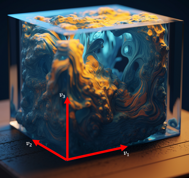
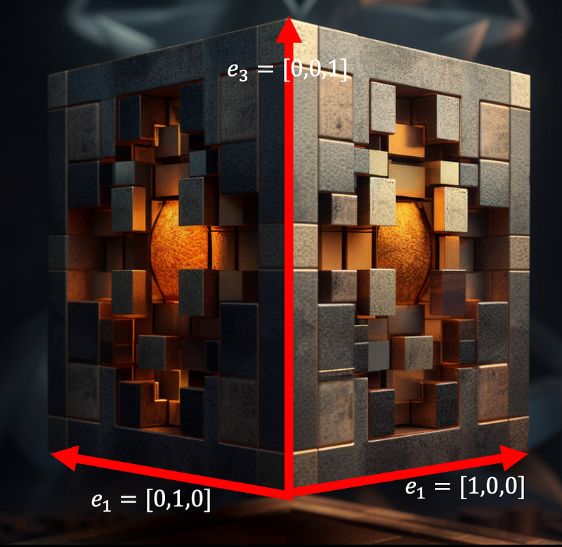
Next, we needed n vectors to form our parallelepiped. Why not take the e1, e2, … en standard basis we defined before. The measure of the patch of space contained between these vectors happens to be 1, by very definition. The picture below for R³ will hopefully make this clear.

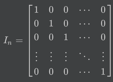
If we collect these vectors from the standard basis into a matrix (rows or columns), we get the identity matrix (1’s on the main diagonal, 0’s everywhere else):

When we said we could apply our linear transform to any n-dimensional patch of space, we might as well apply it to this “standard” patch.

But, it's easy to show that multiplying any matrix with the identity matrix results in the same matrix. So, the resulting vectors after the linear map is applied are the columns of the matrix representing the linear map itself. So, the amount by which the linear map changed the volume of the “standard patch” is the same as the n-dimensional measure of the parallelepiped between the column vectors of the matrix representing the map itself.

To recap, we started by motivating the determinant as the ratio by which a linear map changes the measure of an n-dimensional patch of space. And now, we showed that this ratio itself is an n-dimensional measure. In particular, the measure contained between the column vectors of any matrix representing the linear map.

III) Motivating the basic properties

We described in the previous section how a determinant of a linear map should simply be the measure contained between the vectors of any of its matrix representations. In this section, we use two dimensional space (where measures are areas) to motivate some fundamental properties a determinant must have.

The first property is multi-linearity. A determinant is a function that takes a bunch of vectors (collected in a matrix) and maps them to a single scalar. Since we’re restricting to two-dimensional space, we’ll consider two vectors, both two dimensional. Our determinant (since we’ve motivated it to be the area of the parallelogram between the vectors) can be expressed as:

det = A(v1, v2)

How should this function behave if we add a vector to one of the two vectors? The multi-linearity property requires:

A(v1+v3, v2) = A(v1,v2)+A(v3,v2) __ (1)

This is apparent from the moving picture below (note the new area getting added).

And this visualization can also be used to see (by scaling one of the vectors instead of adding another vector to it):

A(c.v1, v2) = c.A(v1, v2) __ (2)

This second property has an important implication. What if we plug a negative c into the equation? The area, A(v1, v2) should then be the opposite sign to A(c.v1,v2).

Which means we need to introduce the notion of negative area and a negative determinant.

This makes a lot of sense if we’re okay with the concept of negative lengths. If lengths, measures in 1-d space can be positive or negative, then it stands to reason that areas, measures in 2-d space should also be allowed to be negative. And so, measures in space of any dimensionality should as well.

Together, equations (1) and (2) are the multi-linearity property.

Another important property that has to do with the sign of the determinant is the “alternating property”. It requires:

A(v1, v2) = -A(v2, v1) __(3)

Swapping the order of two vectors negates the sign of the determinant (or measure between them). If you learnt about the cross product of 3-d vectors, this property will be very natural. To motivate it, let’s think first of the one-dimensional distance between two position vectors, d(v1, v2). Its clear that d(v1, v2) = -d(v2, v1) since when we go from v2 to v1, we’re traveling in the opposite direction to when we go from v1 to v2. Similarly, if the area spanned between vectors v1 and v2 is positive, then that between v2 and v1 must be negative. This property holds in n dimensional space as well. If in A(v1, v2, …, vn) we swap two of the vectors, it causes the sign to switch.

The alternating property also implies that if one of the vectors is simply a scalar multiple of the other, the determinant must be 0. This is because swapping the two vectors should negate the determinant:

A(v1, v1) = -A(v1, v1)

=> 2 A(v1, v1) = 0

=> A(v1, v1) = 0

We also have by multi-linearity (equation 2):

A(v1, c.v1) = c A(v1, v1) = 0

This makes sense geometrically since if two vectors are parallel to each other, the area between them is 0.

The video [6] covers the geometric motivation of these properties with really good visualizations and video [4] visualizes the alternating property quite well.

IV) Getting algebraic: Deriving the Leibniz formula

In this section, we move away from geometric intuition and approach the topic of determinants from an alternate route. That of cold, algebraic calculations.

See, the multi-linearity and alternating properties which we motivated in the last section with geometry are (remarkably) enough to give us a very specific algebraic formula for the determinant, called the Leibniz formula.

That formula helps us see properties of the determinant that would be really, really hard from the geometric approach or with other algebraic formulas.

The Leibniz formula can then be reduced to the Laplace expansion, involving going along a row or column and calculating co-factors which many people see in high school.

Let’s derive the Leibniz formula. We need a function that takes the n column vectors, 𝛼1, 𝛼2, …, 𝛼n of the matrix as input and converts them into a scalar, c.

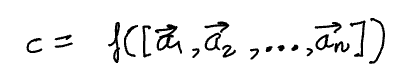
We can express each column vector in terms of the standard basis of the space.

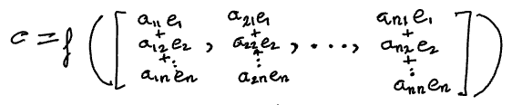
Now, we can apply the property of multi-linearity. For now, to the first column, 𝛼1.

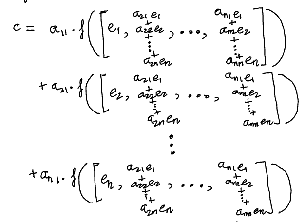
We can do the same for the second column. Let’s take just the first term from the summation above and take a look at the resulting terms.

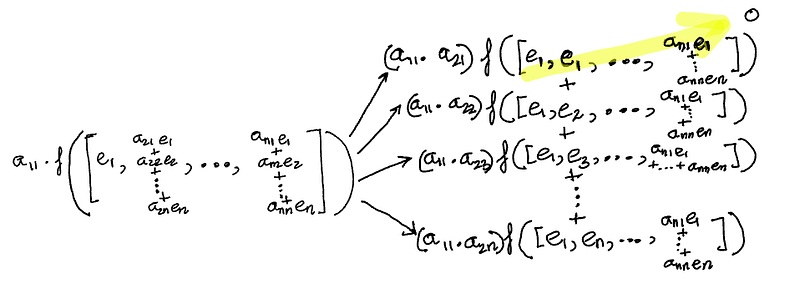
Note that in the first term, we get the vector, e1 appearing twice. And by the alternating property, the function f for that term becomes 0.

In order for two e1’s to appear, the second indices of the two a’s in the product must each become 1.

So, once we do this for all the columns, the terms that won’t become zero by the alternating property will be the ones where the second indices of the a’s don’t have any repetition — so all distinct numbers from 1 to n. In other words, we’re looking for permutations of 1 to n to appear in the second indices of the a’s.

What about the first indices of the a’s? Those are simply the numbers 1 to n in order since we pull out the a_1x’s first, then the a_2x’s and so on. In more compact algebraic notation,

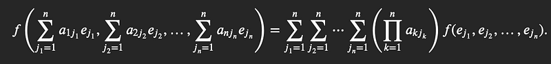
In the expression on the right, the areas, f(e_j1, e_j2, …, e_jn) can either be +1, -1 or 0 since the e_j’s are all unit vectors orthogonal to each other. We already established that any term that has any repeated e_j’s will become 0 leaving us with just permutations (no repetition). Among those permutations, we will sometimes get +1 and sometimes -1.

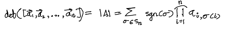
The concept of permutations carries with it signs. The signs of the areas are equivalent to the signs of the permutations. If we denote by S_n the set of all permutations of [1,2,…,n] then we get the Leibniz formula of the determinant:

If you’re still confused about the formula, see the mathexchange post, [3]. And if you’re the kind of person that needs to see working code for things to click, here is some Python:

import numpy as np
import itertools


def permut_sign(a):
    """
    The sign of a permutation is simply the number of inversions.
    This is a simple, O(n^2) algorithm for finding the inversions. It can
    be done more efficiently with merge sort in O(n.log(n)) time.
    """
    cnt = 0
    for i in range(len(a)):
        for j in range(i+1, len(a)):
            if a[i] > a[j]:
                cnt += 1
    # Convert the 0-1 into -1 and +1
    return (cnt % 2 - .5) * -2


def leibniz_determinant(a):
    """
    Here, a is the matrix whose determinant we want to calculate.
    """
    n = len(a)
    arr = np.arange(n)
    determinant = 0
    for perm in itertools.permutations(arr):
        sign1 = permut_sign(perm)
        term = 1
        for i in range(len(perm)):
            j = int(perm[i])
            term = term * a[i, j]
        determinant += sign1 * term
    return determinant


a = np.array([[2, 1, 5],
              [4, 3, 1],
              [2, 2, 5]])

det1 = leibniz_determinant(a)
det2 = np.linalg.det(a)
print(abs(det1 - det2) <= 0.00001)

One shouldn’t actually use this formula to calculate the determinant of a matrix (unless it’s just for fun or exposition). It works, but is comically inefficient given the sum over all permutations (which is n!, superexponential).

However, many theoretical properties of the determinant become trivial to see with the Leibniz formula when they would be very hard to decipher or prove if we started from another of its forms. For example:

1. With this formula it becomes apparent that a matrix and its transpose have the same determinant: |A| = |A^T|. It’s a simple consequence of the symmetry of the formula.
2. A very similar derivation to the above can be used to show that for two matrices A and B, |AB| = |A|.|B|. See this answer in the mathexchange post, [8].
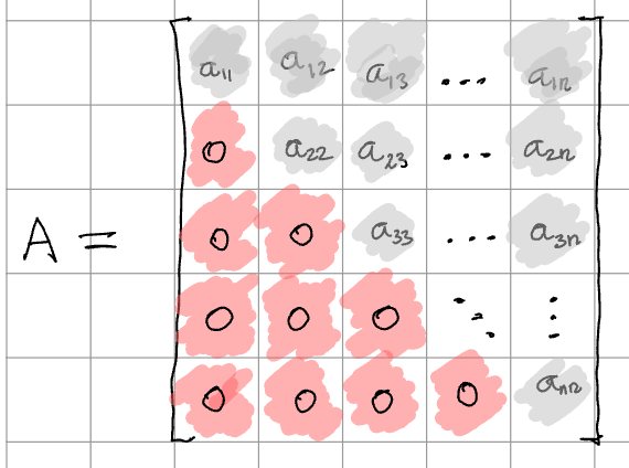
3. With the Leibniz formula, we can easily see that if the matrix is upper triangular or lower triangular (lower triangular means every element of the matrix above the diagonal is zero), the determinant is simply the product of the entries on the diagonal. This is because all permutations bar one: (a_11.a_22…a_nn) (the main diagonal) get some zero term or the other and make their terms in the summation 0.

The third fact actually leads to the most efficient algorithm for calculating a determinant that most linear algebra libraries use. A matrix can be decomposed efficiently into lower and upper triangular matrices (called the LU decomposition which we’ll cover in the next chapter). After doing this decomposition, the third fact is used to multiply the diagonals of those lower and upper matrices to get their determinants. And finally, the second fact is used to multiply those two determinants and get the determinant of the original matrix.

A lot of people in high school or university when first exposed to the determinant, learn about the Laplace expansion, which involves expanding about a row or column, finding co-factors for each element and summing. That can be derived from the above Leibniz expansion by collecting similar terms. See this answer to the mathexchange post, [2].

V) Historic motivation

The determinant was first discovered in the context of linear systems of equations. Say we have n equations in n variables (x_0, x_1, …, x_n).

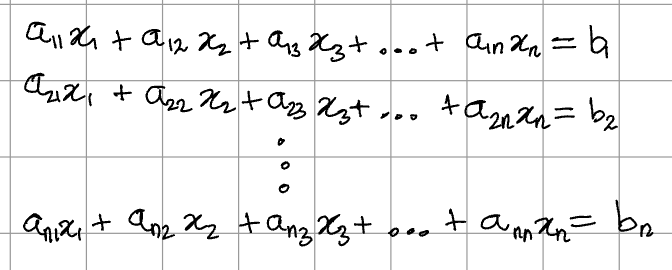
This system can be expressed in matrix form:

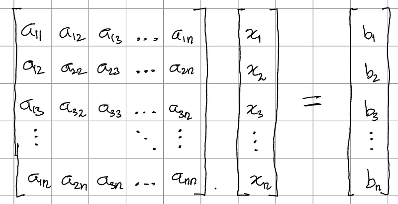
And more compactly:

A.x = b

An important question is whether or not the system above has a unique solution, x. And the determinant is a function that “determines” this. There is a unique solution if and only if the determinant of A is non-zero.

This historically inspired approach motivates the determinant as a polynomial that arises when we try to solve a linear system of equations associated with the linear map.

For more on this, see the excellent answer in the mathexchange post, [8].

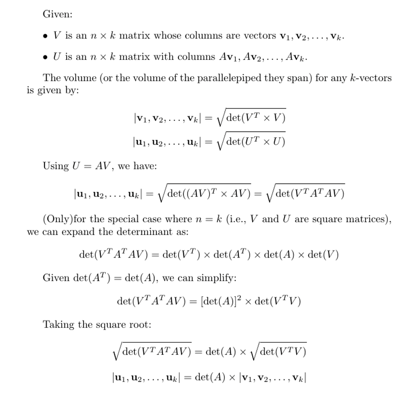
VI) Proof of the property we motivated with

We started this chapter by motivating the determinant as the amount by which the R^n to R^n linear map changes the measure of an n-dimensional patch of space. We also said that this doesn’t work for 1, 2, .. n-1 dimensional measures. Below is a proof of this where we use some of the properties we encountered in the rest of the sections.

If you’re enjoying the book, consider buying me a coffee for motivation :)

https://www.buymeacoffee.com/w045tn0iqw

References

[1] Mathexchange post: Determinant of a linear map doesn’t depend on the bases: https://math.stackexchange.com/questions/962382/determinant-of-linear-transformation

[2] Mathexchange post: Determinant of a matrix Laplace expansion (high school formula) https://math.stackexchange.com/a/4225580/155881

[3] Mathexchange post: Understanding Leibniz formula for determinants https://math.stackexchange.com/questions/319321/understanding-the-leibniz-formula-for-determinants#:~:text=The%20formula%20says%20that%20det,permutation%20get%20a%20minus%20sign.&text=where%20the%20minus%20signs%20correspond%20to%20the%20odd%20permutations%20from%20above.

[4] Youtube video: 3B1B on determinants https://www.youtube.com/watch?v=Ip3X9LOh2dk&t=295s

[5] Connecting Leibniz formula with geometry https://math.stackexchange.com/questions/593222/leibniz-formula-and-determinants

[6] Youtube video: Leibniz formula is area: https://www.youtube.com/watch?v=9IswLDsEWFk

[7] Mathexchange post: product of determinants is determinant of product https://math.stackexchange.com/questions/60284/how-to-show-that-detab-deta-detb

[8] Historic context for motivating determinant: https://math.stackexchange.com/a/4782557/155881