A Beautiful Way of Looking at Linear Regressions

Once you see it, your previous ideas will be just projections

Did you know that linear regressions are orthogonal projections? This is obvious for mathematicians but simple minds like yours and mine might have never thought about it. We can still appreciate the beauty of this though. Knowing that every linear regression can be visualized as a problem in space is a game-changer. Don’t feel bad if you didn’t know this. You still have the chance of having a mind-blowing experience for the first time.

What is the method of least squares and why should you care?

The method of least squares is one of the most used methods in data fitting. It allows you to take a bunch of data and come up with a mathematical expression that models the behavior of that data. If you think that this has nothing to do with you, you might be wrong. The least squares are not only for mathematicians and engineers. Least squares are everywhere and belong to everyone. They are immersed in your phone preferences, your Netflix account, and your daily life. Everywhere you look, data is being collected and used to build models that represent the behavior of that data and predict what the next step should be. Even if these models are more complicated than what we are going to explain here, the basic aspects of the least squares remain.

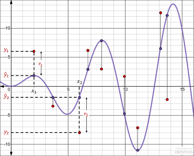
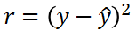
Figure 1. Differences between modeled and observed data. Graph made by the author in desmos and previously used here.

This might be the simplest explanation of the method of least squares: we have some input data x that is responsible for some output data y. Our goal is to find a mathematical expression that evaluates x and results in a ŷ that is as closest as possible to y. Figure 1 shows some data points in red and a curve in purple. The data points are the observed data we are trying to match. The purple curve is the mathematical model that we build to represent the behavior of the red dots. Note how we can calculate the differences between the observed values (y) and the modeled ones (ŷ). These differences are represented with the letter r. Once again, our goal is to find a model where r is as small as possible. However, we have a problem: r could be negative or positive depending on how we calculate it. To solve this, we are not going to calculate r as y-ŷ or ŷ-y. Our calculation will be:

If we calculate the square of the differences between y and ŷ, the result will always be positive. Then, the method of the least squares consists of finding the model where the square of the differences between the observed and the modeled data is as small as possible.

The traditional explanation

The difference between observed and modeled data is often called residual and mathematically is expressed by:

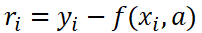
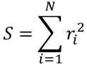
Note how ŷ is a function f that is evaluated for each xi using the coefficients a. Finding these coefficients is our main objective. Ideally, we would like to know which are the coefficients that take us to the minimum possible value of S.

To find the minimum of S we can set the gradient to zero and find the coefficients a. If you are not clear about how you can find a minimum when the gradient equals zero, you can visit this article (particularly the section “A graphical explanation for the minimization of a function using derivatives”).

In linear regressions problems, the application of the method of least squares always has a unique solution which is not the case for non-linear regressions. The solution for the linear problem is presented in the following equation whose explanation can be found in multiple books and web pages.

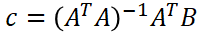
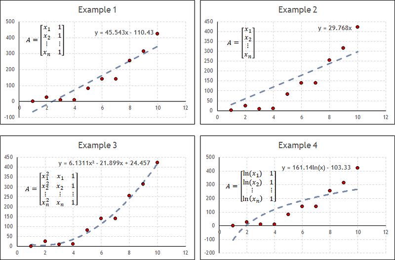
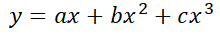
The main thing to understand here is that the vector c contains the coefficients for the linear expression that models the data. This vector is a function of the observed values (B), the input values (A), and the type of expression that we want to use as a model. The following picture shows four examples of linear regressions using the same input data but changing the type of model or equation. Each column of A represents one term of the equation and each row represents the input values. Note how c will always be a matrix with a single column and a number of rows equal to the number of parameters we are defining. The equations contained in each plot represent the best possible mathematical representation of the data for each model.

Figure 2. Examples of linear regressions using the same input data but changing the mathematical model. Graph made by the author.

Take another look

In all the examples from the previous picture, we had one variable for input data (x) and one for output data (y). However, we could have worked with more than one variable for the input data. We could have a function such as:

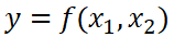
Equation 5. Model that depends on two independent variables

In this case, instead of obtaining a line that describes the best possible match between our model and the data, we could obtain a surface. If we keep adding more variables to our input data, we could find more coefficients for the best possible fit. So least squares and linear regression are not only applicable for the plots in Figure 2, you could apply this methodology to find a mathematical model that represents multiple independent variables.

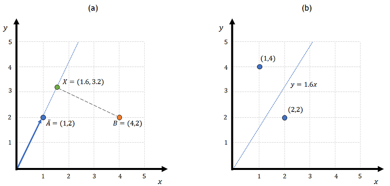
When applying the least squares method to linear regressions we can think of it differently. Let’s imagine that we have a vector a that is represented by the blue line in Figure 3a. The position of this vector is also marking the position of a line in the xy plane (thin dotted blue line). Now let’s say that we want to find what is the closest point in that line to another point in the plane, in this case, B. This is similar to asking what is the minimum distance between B and the blue line. This minimum distance corresponds to the orthogonal projection of B on the line. Figure 3b shows a point X that represents this projection. As you can see, the green line that goes from B to X forms 90 degrees with the blue line which means that X is the orthogonal projection of B on the blue line.

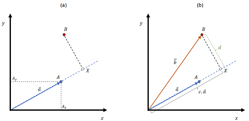
Figure 3. (a) Orthogonal projection of point B onto the line defined by vector A. (b) Distance from point B to its orthogonal projection. Graphs made by author.

The question now is: how can we find X? Figure 3b shows that there is a constant C that multiplies the vector a such that the position of A is now the value we are looking for. So the question of finding X can be solved by determining a c that multiplied by a will minimize the distance from B to the blue line.

The first thing to do is find a way of calculating the distance d between B and A. One way of doing this is using the Euclidean distance between these points. We can calculate this distance as follows:

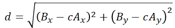
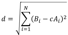
Equation 6. Euclidean distance between 2 points in 2 dimensions

Note that Bx, Ax, By and Ay correspond to the coordinates of the points A and B in the x and y axis. This is one of the cool features of this type of distance calculation. For this example, we are calculating the distance between two points on a plane. We can also calculate the distance between two points in space and we can even calculate the distance between points in 10-dimensional space. The equation is always the same and can be written as follows (where N represents the number of dimensions):

Equation 7. Euclidean distance between any number of points in an N-dimensional space

We have a way of calculating the distance between B and A. What we need now is to find which c will minimize this distance. You know what to do, right? Let’s differentiate the equation with respect to c and set it equal to zero. Before doing that, it is very important to realize that calculating the minimum of eq. 7 is the same as calculating the minimum of:

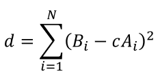
Equation 8. Sum of the squares of the distance between multiple points in each dimension

This is due to the monotonicity of the square root function. Don’t be scared by the name. That just means that finding the minimum of the square root of a function is actually finding the minimum of the argument of the square root of a function. If someone asks you which is a smaller number √5 or √6, you could quickly say 5 since the square root function is monotonic.

Going back to our discussion, the goal is to take eq. 8 and calculate c such that d is minimum. If we differentiate this equation we will get:

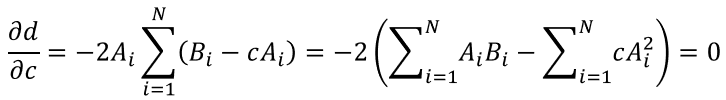
Equation 9. Differentiating eq.8 and setting it equal to zero

The summations contained in eq. 9 can be substituted if we work with matrices instead of single values. Let’s say that A represents an array of the values of A in all dimensions (in a 2D problem this would mean Ax and Ay) and B represents another array with the values of B in all dimensions. Then we can express the previous equation as:

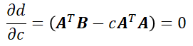
Remember that, to multiply matrices, the number of columns from the first matrix need to match the number of rows of the second one. That is why to multiply A times B or A times A we need to calculate the transpose of A.

From the previous expression we can obtain c, which is:

Equation 11. Vector c that minimized the distance d between the point B and the line defined by vector A

This value of c is what we were looking for and is (surprisingly maybe?) what we used before in eq.4 . What does this mean? From a projection point of view, c represents the place on the line defined by vector a where the orthogonal projection of point B is located (Fig. 3). From a linear regression point of view, c represents the coefficients that multiplied by each row in A will lead you to the best possible representation of the input data (Fig. 2). These might seem like two completely different things but they are actually connected. When we are doing a linear regression we are finding a linear combination of the functions contained in each of the rows in A. In the example of the line, there is only one row in A so finding the linear combination of this single function is actually finding the projection of B on the line.

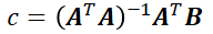
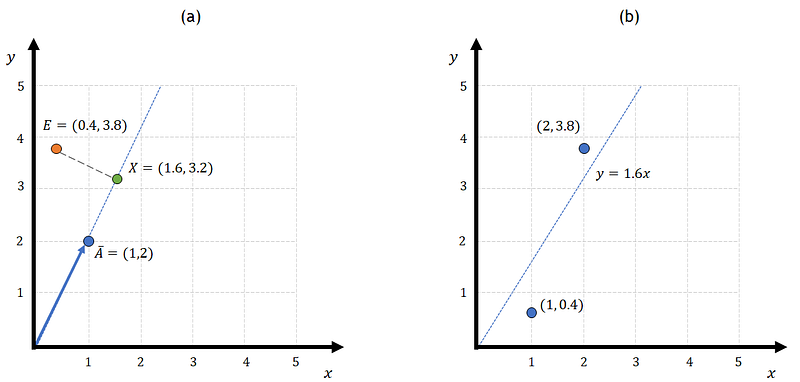
It is time for an example! Let’s say that we want to calculate the projection of point B=(4,2) on a line defined by vector A=(1,2) as it is shown in Fig. 4. For this case, we can define a matrix A and a matrix B and calculate c with the expression we found on eq. 11.

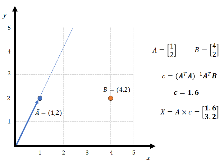
Figure 4. Example of the calculation of the projection of point B in the line defined by vector A. Graph made by author.

The position of the projection of B on the line is X=A.c which is (1.6, 3.2). So, what does this have to do with linear squares? Let’s say that instead of reading A and B as two points we read them as a pair of input/target data. In that case, we would have two data points: (1,4) and (2,2) that we want to fit a model using linear regression. As Fig. 5 shows, the linear regression coefficient that we find is also 1.6. This means that performing a linear regression is like finding the orthogonal projection of a target vector onto a subspace that is formed by each of the functions we want to include in the regression. In this case, point (4,2) was projected into the subspace formed by vector (1,2). This is like example 2 on Fig. 2 where the matrix A that defines the elements of the linear regression, only had values for [x1, x2,…xn].

Figure 5. (a) Projection of point B on the line defined by vector A. (b) Linear fit of points (1,4) and (2,2). Graphs made by the author.

Yes, linear regression is an orthogonal projection and, once you see it, everything makes sense. We can even take the previous example, find another point E that has the same orthogonal projection, and notice that the linear regression coefficient is the same (Fig. 6). In this case, the data points are closer to the line so R² will increase. However, the slope is exactly the same for both cases. We can find an infinite combination of points that are adjusted with the same regression coefficient since there is an infinite number of points whose orthogonal projection is X. Have you heard about Anscombe’s quartet? Now is a good time to take a look at it.

Figure 6. (a) Projection of point E on the line defined by vector A. (b) Linear fit of points (1,0.4) and (2,3.8). Graphs made by the author.

A leap into the third dimension

So far the examples we have seen only contain 2 data points. There is a reason for that. Having N data points means that the vector we want to project is N-dimensional which is difficult to visualize. Let’s say that we have a set of 100 data points that we want to adjust to a linear regression of the form:

Equation 12. Example of a linear expression with 3 coefficients

In this case, we would have a 100-dimensional vector that we want to project onto a 3-dimensional space. Can you visualize this? Maybe it is too much. Let’s use a simpler example: we have a data set of 3 points that we want to adjust using linear regression with two coefficients. This is shown in Figure 7.

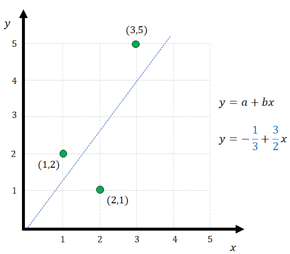
Figure 7. Linear regression with the type y=a+bx for a dataset of 3 points. Graph made by the author.

If we apply linear regression to the previous example we will find that the best fit occurs when a=-⅓ and b=3/2. How can we represent this in 3-dimensional space? For this case, we have a target vector t=[2,1,5] that we want to project onto a surface formed by vectors A=[1,1,1] and B=[1,2,3]. Remember that the expression we are looking for has a coefficient that multiplies x (vector A) and a bias or a coefficient that is multiplying 1 (vector B). Take a look at Fig. 8.

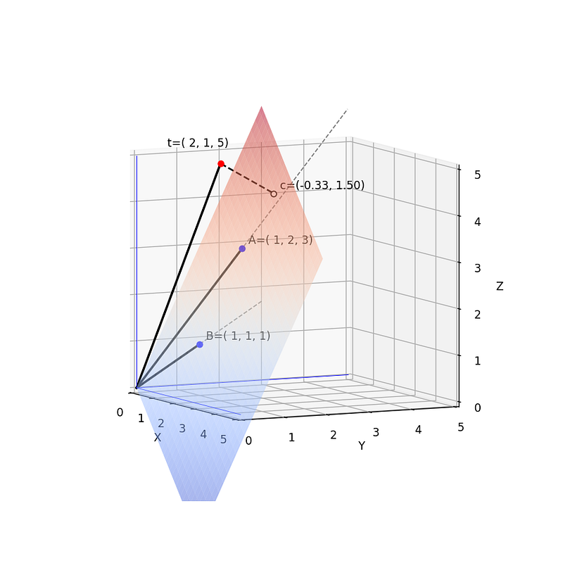
Figure 8. Projection of point t onto the subspace formed by vectors A and B. Graph made by author using this Python notebook.

Point c represents the orthogonal projection of the target vector t onto a surface that is formed by the vectors that define the linear regression. The reason why c is (-0.33, 1.5) is that if we imagine a 2D coordinate system formed by B=(1,1,1) as the y-axis and A=(1,2,3) as the x-axis, c is negative in y and positive in x. If we change the position of the point we want to project, we will see that its position on the 2D-subspace changes accordingly (Fig.9).

Figure 9. Projection of point t2 onto the subspace formed by vectors A and B. Graph made by author using this Python notebook.

Similar to what we did before, we can now find an infinite number of points whose projection on the plane is also c. This means that these points will be adjusted with the same linear regression coefficients although the distance from the points to the model will change. If you want to play with different points and planes you are welcome to use this Python notebook that I uploaded to GitHub. I tried to explain as much as I could about what I did in each part of the code.

After the previous example, it might be easier to imagine a situation where we want to project a point that belongs to a 100-dimensional space into a 2-dimensional space formed by 2 vectors. It is hard to have a clear picture of how this 100-dimensional space would look like but, if we extrapolate what we did before, there is no doubt that we will find a point in a 2D space that represents the orthogonal projection of the original point in the 100-dimensional space. This article by Prof. John D. Norton from the University of Pittsburgh contains a great explanation of how to visualize things in 4 dimensions. I will leave the picture of the point in the 100-dimensional space to your imagination!

Conclusions

What is written in this article is not new. As I said in the introduction, if you are a mathematician, the chances are that all this is obvious to you. However, the reason why I decided to write this is that, after running multiple linear regressions in different programs, I never took a pause to think about what I was actually doing. When I realized that linear regressions were actually orthogonal projections I felt that I finally understood what I had been doing for years without thinking. This helped me to realize why linear regressions are problems with close solutions and why in some cases they are not such a good idea. In any case, and regardless of your mathematical knowledge, I hope you find this as interesting as I found it some days ago while looking through my old linear algebra book.

References

Vladimir Mikulik (2017). Why Linear Regression is a Projection.
Thomas S. Robinson (2020). Fundamental Theorems for Econometrics. Chapter 3.
John D. Norton (2001). What is a four dimensional space like?
Christopher M. Bishop (2006) Pattern Recognition and Machine Learning. Springer.