Even SQL Newbies Can Materialize SQL Views In Under 10 Minutes

Learn one of the most useful but intimidating SQL/data engineering skills in just a few minutes.

Materialize Your SQL Views With No Fear

Before you get intimidated by a technical sounding phrase like “materializing views”, I want to assure you that this is a fancy way to express a very simple concept.

Materializing a view = creating a table.

Of course, this table isn’t created from nowhere. Because the source material, your view, is already created, materializing a view is more of a conversion exercise; you’re not starting from scratch.

Since views are just saved queries, you already have the building blocks of a table: Schema, partitioning and a sample of data to be included in the final view/table.

Having existing elements to work off of makes materializing a table one of the easier tasks you’ll tackle as a data engineer.

Obviously you still need to apply best practices, conduct quality assurance and be careful not to break existing infrastructure, but you have a “head start” that will pay dividends during development.

Below, we’ll walk through a simple materialization, covering:

Materialization methods
Materialization use cases
Materialization scheduling/orchestration

You already have the building blocks for a materialized view. Photo by Xavi Cabrera on Unsplash.

SQL View Materialization In Google Cloud Platform

Your method of materialization will depend largely on your tech stack.

For instance, I use a Google Cloud (GCP)-based tech stack so when I materialize a table, I convert a query to a recurring process like a cloud function. If the table is dependent on other upstream processes or sources I might build out a more complex process like an Airflow DAG.

However, if you use a dbt-based stack you already have a leg up due to the fact you can specify a materialization preference when creating a model. For the purposes of this walkthrough, I’ll be covering a GCP implementation.

To materialize a view using a Google Cloud Function, you’ll want to begin with the query that creates the view. For those new to views, the query that creates a view is called a view definition.

In BigQuery, you can see the underlying view definition by clicking “Details” after clicking on a table.

For this example, I’ll materialize a view I used in a previous piece to demonstrate the concept of flattening a nested table.

Flattening Your SQL Tables — Not As Easy As It Sounds

How to expose deeply nested SQL fields — and why you need to be careful when handling complex raw data.

medium.com

Here is the query in its entirety:

SELECT
  object_id,
  logoAnnotations,
  l_a.properties,
  l_a.locations,
  l_a.boundingPoly,
  l_a.topicality,
  l_a.confidence AS label_confidence,
  ROUND(l_a.score, 2) AS score,
  l_a.description,
  l_a.locale,
  l_a.mid,
  ch.importanceFraction,
  ch.confidence,
  b_v.x,
  b_v.y
FROM
  `bigquery-public-data.the_met.vision_api_data`,
  UNNEST(labelAnnotations) l_a,
  UNNEST(cropHintsAnnotation.cropHints) ch,
  UNNEST(ch.boundingPoly.vertices) b_v

From here, your approach is up to personal preference. You could convert your existing query to DML using DELETE or CREATE OR REPLACE and INSERT followed by the query you saved as a view.

This would be my approach if I were incorporating this query as a task in a DAG because you can use a class like BigQueryOperator to write to a table on a recurring basis.

Pardon the interruption: For more Python, SQL and cloud computing walkthroughs, follow Pipeline: Your Data Engineering Resource.

To receive my latest writing, you can follow me as well.

Use A Cloud Function To Materialize A SQL View

For a cloud function I like just taking the original query and, provided it’s not super compute-intensive, then I convert it to a data frame.

from google.cloud import bigquery
import pandas

bq_client = bigquery.Client()

query = """

SELECT
  object_id,
  logoAnnotations,
  l_a.properties,
  l_a.locations,
  l_a.boundingPoly,
  l_a.topicality,
  l_a.confidence AS label_confidence,
  ROUND(l_a.score, 2) AS score,
  l_a.description,
  l_a.locale,
  l_a.mid,
  ch.importanceFraction,
  ch.confidence,
  b_v.x,
  b_v.y
FROM
  `bigquery-public-data.the_met.vision_api_data`,
  UNNEST(labelAnnotations) l_a,
  UNNEST(cropHintsAnnotation.cropHints) ch,
  UNNEST(ch.boundingPoly.vertices) b_v

"""

mt_vision_df = bq_client.query().to_dataframe()

I like simple data frame conversions because I can easily do transformations in the script without having to touch the underlying query. It’s a matter of personal preference but I prefer Pandas for conversion operations like converting to datetime or integer and SQL for other data-oriented operations.

In this case, I’m much more comfortable doing the unnest operations in the query itself rather than using a Pandas method like read_json or from_dict.

Once you’ve configured a BigQuery client to load the underlying view definition, then you’re more than halfway finished materializing your view.

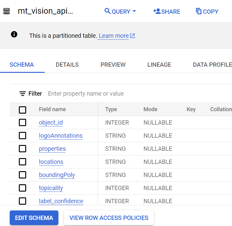
Before we can upload to BigQuery, we need to pass a schema to the BigQuery load function. Luckily, because the table will be based on the existing view’s schema, we already know the schema we want to include.

I can get the existing schema by querying the metadata of the view, downloading the JSON response, and specifying it in the body of my script (or my config file).

SELECT 
column_name AS name, 
CASE WHEN data_type = "INT64" THEN "INTEGER"
     WHEN data_type = "ARRAY<STRING>" THEN "STRING"
     WHEN data_type = "FLOAT64" THEN "FLOAT"
ELSE data_type END AS type,
"NULLABLE" AS mode
FROM `ornate-reef-332816.sample_dataset.INFORMATION_SCHEMA`.COLUMNS
WHERE table_name = "vision_api_flattened"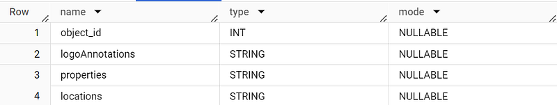

Schema as a BigQuery table. Screenshot by the author.

We can create a schema and table from the JSON that underlies this table output. Here’s what the newly materialized table looks like:

Table details page showing schema. Screenshot by the author.

Full Python Script & Final Implementation

Passing the schema to the load function is one of the final steps in writing the Python script.

from google.cloud import bigquery
import pandas

dataset = "sample_dataset"
table = "mt_vision_api_results"

bq_client = bigquery.Client()

def upload_to_bq(df: pd.DataFrame, dataset_id: str, table_id: str, write_dispo: str, schema: list):
    
    dataset_ref = bq_client.dataset(dataset_id)
    table_ref = dataset_ref.table(table_id)

    job_config = bigquery.LoadJobConfig()
    job_config.write_disposition=write_dispo
    job_config.source_format = bigquery.SourceFormat.CSV
    job_config.schema = schema
    job_config.ignore_unknown_values=True 

    job = bq_client.load_table_from_dataframe(
    df,
    table_ref,
    location='US',
    job_config=job_config)
    
    return job.result()

def main(event, context):

  query = """

  SELECT
    object_id,
    logoAnnotations,
    l_a.properties,
    l_a.locations,
    l_a.boundingPoly,
    l_a.topicality,
    l_a.confidence AS label_confidence,
    ROUND(l_a.score, 2) AS score,
    l_a.description,
    l_a.locale,
    l_a.mid,
    ch.importanceFraction,
    ch.confidence,
    b_v.x,
    b_v.y
  FROM
    `bigquery-public-data.the_met.vision_api_data`,
    UNNEST(labelAnnotations) l_a,
    UNNEST(cropHintsAnnotation.cropHints) ch,
    UNNEST(ch.boundingPoly.vertices) b_v
  
  """

  schema = 

  [{
  "name": "object_id",
  "type": "INTEGER",
  "mode": "NULLABLE"
}, {
  "name": "logoAnnotations",
  "type": "STRING",
  "mode": "NULLABLE"
}, {
  "name": "properties",
  "type": "STRING",
  "mode": "NULLABLE"
}, {
  "name": "locations",
  "type": "STRING",
  "mode": "NULLABLE"
}, {
  "name": "boundingPoly",
  "type": "STRING",
  "mode": "NULLABLE"
}, {
  "name": "topicality",
  "type": "INTEGER",
  "mode": "NULLABLE"
}, {
  "name": "label_confidence",
  "type": "INTEGER",
  "mode": "NULLABLE"
}, {
  "name": "score",
  "type": "FLOAT",
  "mode": "NULLABLE"
}, {
  "name": "description",
  "type": "STRING",
  "mode": "NULLABLE"
}, {
  "name": "locale",
  "type": "STRING",
  "mode": "NULLABLE"
}, {
  "name": "mid",
  "type": "STRING",
  "mode": "NULLABLE"
}, {
  "name": "importanceFraction",
  "type": "FLOAT",
  "mode": "NULLABLE"
}, {
  "name": "confidence",
  "type": "FLOAT",
  "mode": "NULLABLE"
}, {
  "name": "x",
  "type": "INTEGER",
  "mode": "NULLABLE"
}, {
  "name": "y",
  "type": "INTEGER",
  "mode": "NULLABLE"
}]
  
  mt_vision_df = bq_client.query().to_dataframe()

  upload_to_bq(mt_vision_df, dataset, table, schema)

if __name__ == "__main__":
  main("","")

After your Python script is complete, we’ll need to schedule the view to load on a recurring basis. Remember that a view loads each time it’s queried and for connected visualization tools like Looker Studio, it refreshes automatically on frequent intervals (in Looker’s case, every 15 minutes).

When you convert your view to a “regular” table, then you’ll need to be precise in how you specify its load interval.

The loading frequency should depend on the data the table contains.

Ask yourself:

How often is this data refreshed? Daily? Weekly?
Who consumes this data and what are their timing expectations?
What upstream processes does this data depend on and when is this data typically available?

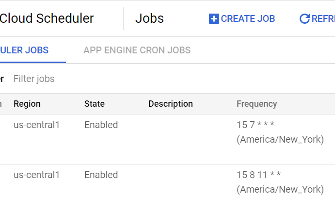
Then you can use a tool like cloud scheduler (event-based trigger written in cron) to load your new table.

Keep This In Mind When Materializing Your Views

The biggest motivator to materialize a view is control.

By converting a view to a table and creating an associated loading mechanism, you can control when and how this data is loaded.

Since views can’t be overwritten or used with DML, converting to a table allows you to do operations like type conversions and you can now drop columns or edit the underlying schema.

These advantages have to be weighed against the increased storage burden you create when you convert a saved query to a permanent table. Depending on the size and scale of the data you maintain this may or may not be the most sustainable and cost-effective option.

Ultimately, determining whether to materialize a view is like any other decision regarding your data infrastructure.

You need to think not just about the new data source you’re building, but also how such a transition would impact existing data sources and infrastructure.

Materializing a table gives you control but it also leaves you with a lot of decisions.

Create a job-worthy data portfolio. Learn how with my free project guide.