
Experiment Analysis
Decoding Data Success: A Comprehensive Guide to A/B Testing Analysis [Part 3]
Discover advanced DID and Multivariate Testing strategies, redefining precision in outcome decoding.
Welcome to the third chapter of our deep dive into the world of experimental analysis, where we untangle the complexities of A/B testing and illuminate the path to data-driven decision-making.
In this installment, we move beyond the foundational concepts into advanced techniques that add a layer of sophistication to our analytical understanding. Join us on this journey as we dissect the Difference-in-Difference (DID) method and Multivariate Testing (A/B/n Tests) unlocking insights into experimental outcomes.
The comprehensive analysis is presented across a series of three blogs, with each installment delving into the specifics of individual steps. This blog is Part 3 of the series. Kindly refer to Part 1 and Part 2 for the foundations of the series.

Before we plunge into the depths of advanced methodologies, let’s reflect on the ground we’ve covered. In the earlier segments, we meticulously explored the essentials of A/B testing, breaking down the crucial steps for a robust analysis. Now, in Part 3, we ascend to a higher plane, addressing scenarios where traditional methods fall short and demand a more nuanced approach.
Difference-in-difference method
Difference-in-difference method is used when sampling bias exists in the A/B experiment setup. In this case, we can not use generic T-test or Mann-Whitney U test methods.
Difference-in-difference holds a key assumption, which is called a parallel-trend assumption. The parallel-trend assumption states that if no treatment had occurred, the difference between the treated group and the untreated group would have stayed the same in the post-treatment period as it was in the pre-treatment period.
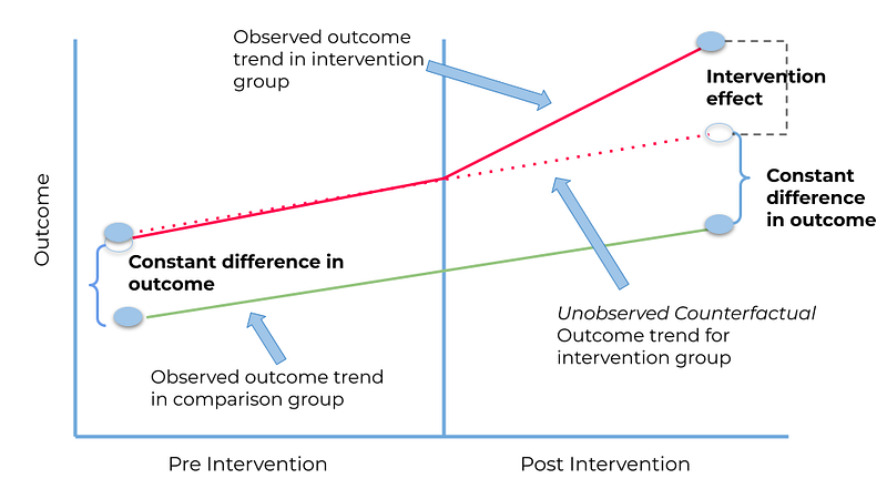
The approach removes biases in post-intervention period comparisons between the treatment and control group that could be the result of permanent differences between those groups, as well as biases from comparisons over time in the treatment group that could be the result of trends due to other causes of the outcome.
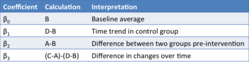
DID is usually implemented as an interaction term between time and treatment group dummy variables in a regression model.
Y= β0 + β1*[Time] + β2*[Intervention] + β3*[Time*Intervention] + β4*[Covariates] + ε
import pandas as pd
from patsy import dmatrices
import statsmodels.api as sm

df = pd.read_csv('us_fred_coastal_us_states_avg_hpi_before_after_2005.csv')
reg_exp = 'HPI_CHG ~ Time_Period + Disaster_Affected + Time_Period*Disaster_Affected'

y_train, X_train = dmatrices(reg_exp, df, return_type='dataframe')
did_model = sm.OLS(endog=y_train, exog=X_train)
did_model_results = did_model.fit()
did_model_results.summary()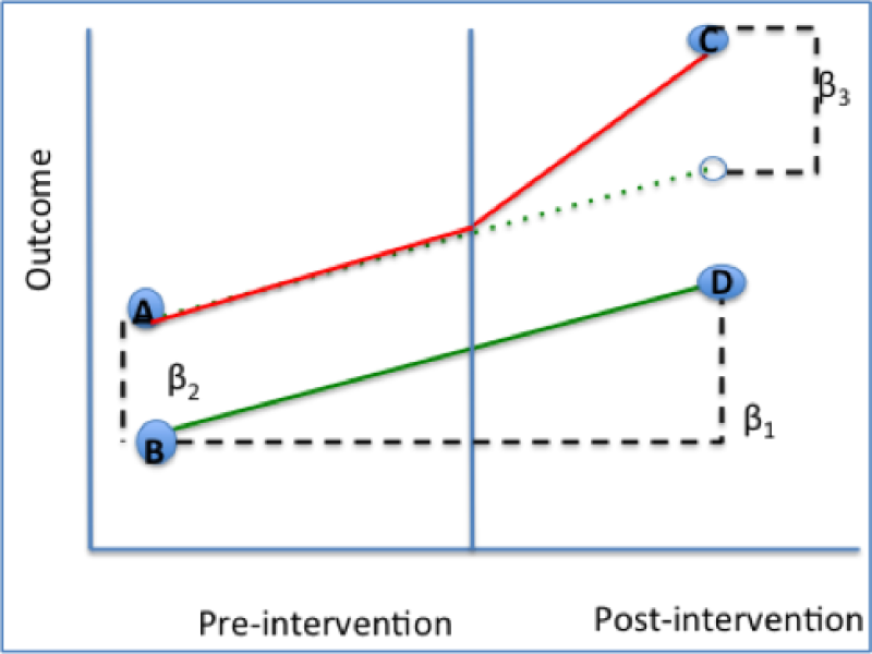
Multivariate Test (A/B/n Test)
A/B/n testing is a type of testing where multiple versions are compared against each other to determine which has the most impact. In this type of test, traffic is split randomly and evenly distributed between the different versions of the page to determine which variation performs the best.
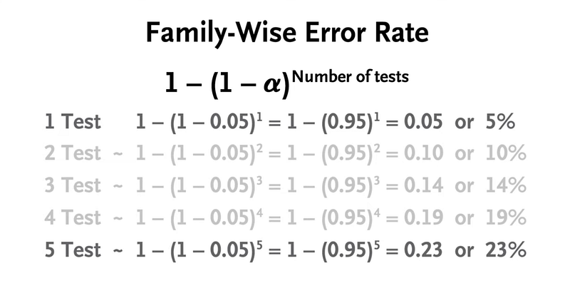
However A/B/n testing leads to an increase in false-positive results. For instance, let’s say we have nine variants, and a statistical significance threshold is set to 0.05. In that scenario, the probability of getting a false-positive result will increase to 0.37. The probability can be calculated using the formula given below:
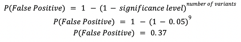
This is known as the Problem of Multiple Comparisons or Alpha Inflation.
Hence we need to correct P values to handle Alpha Inflation.
P Value Correction for MVT
We can perform Benjamini-Hochberg (BH) correction to correct P values. The method ranks the P-value from the lowest to the highest and then adjusts the P-value of each variant accordingly.
BH correction used the rank & number of variants to correct the P value-
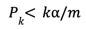
Where k is the rank and m is the number of variants. This approach is less conservative than the Bonferroni correction, which has the same impact on alpha value for all the variants.
Executing the Benjamini–Hochberg Procedure:
- Arrange individual p-values in ascending order.
- Assign ranks to each p-value, starting from 1 for the smallest.
- Calculate the Benjamini-Hochberg critical value for each p-value using the formula (i/m)Q, where i is the rank, m is the total number of tests, and Q is the chosen false discovery rate.
- Compare original p-values to the critical values obtained; identify the largest p-value smaller than the critical value.
As an example, a subset of 25 test results is displayed, featuring corresponding p-values in column 2. Following the ordering (Step 1) and ranking process (Step 2) presented in column 3, the calculation for critical values at a 25% false discovery rate is depicted in column 4 (Step 3). For example, the critical value for item 1 in column 4 is computed as (1/25) * .25 = 0.01, offering clarity on the result assessment.
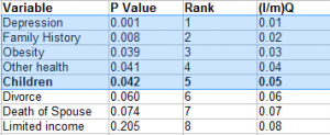
The bolded p-value marks the highest value smaller than the critical threshold (e.g., .042 < .050). All values surpassing it, despite having lower p-values, are highlighted and deemed significant. For instance, while Obesity and Other Health may seem insignificant initially (e.g., .039 > .03), the Benjamini-Hochberg correction renders them significant. In essence, rejecting the null hypothesis for these values is required after correction.
Optional Reading
Bonferroni Correction
The Bonferroni correction counteracts the family-wise error rate problem by adjusting the alpha value based on the number of tests.
To find your adjusted significance level, divide the significance level (α) for a single test by the number of tests (n).
Bonferroni correction = α / n
For example, if your original, single test alpha is 0.05 and you have a set of five hypothesis tests, your adjusted significance level is 0.05 / 5 = 0.01. Your results are statistically significant when your p-value is less than or equal to the adjusted significance level.
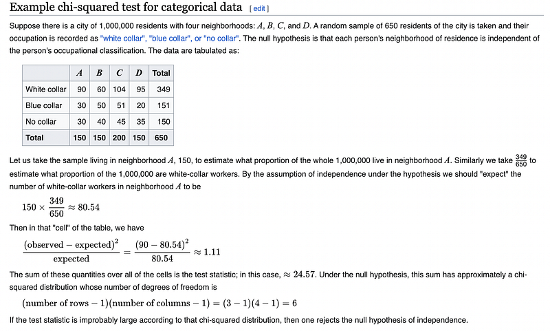
Chi-Square Test
The chi-square test is primarily used to examine whether two categorical variables are independent in influencing the test statistic.
As we draw the final curtain on this comprehensive exploration of A/B testing analysis, our journey traverses beyond statistical fundamentals into the realm of advanced methodologies that redefine precision and insight. Recapping our voyage, we dissected AB testing in its foundational glory, addressed sampling bias with the Difference-in-Difference method, and handled the challenge of false positives through P value correction
To those who have journeyed with us through these three parts, a sincere thank you for your engagement. I invite you to connect on LinkedIn for continued discussions and wish you the utmost success in your data-driven endeavors.
Happy experimenting!
References
- https://en.wikipedia.org/wiki/Difference_in_differences
- https://hkspra.org/product_image_pub/130_580869.pdf
- https://en.wikipedia.org/wiki/Chi-squared_test
If you have read so far, a big thank you for reading! I hope you find this article to be helpful. If you’d like, add me on LinkedIn!
Good luck this week, Pratyush