
Experiment Analysis
Decoding Data Success: A Comprehensive Guide to A/B Testing Analysis [Part 2]
Explore statistical rigour in A/B testing, from significance tests to post-test computations for data-driven success
Step into the second chapter of our guide, where the journey deepens into the heart of A/B experiment analysis. Having established a solid foundation with sanity checks and variance reduction techniques in Part 1, we now embark on an exploration of Statistical Tests. This phase is pivotal, as it unveils the significance of the variations introduced in our experiments, emphasizing precision and rigour in our quest for data-driven success. Let’s navigate through the statistical landscape, unravelling the process for informed decision-making.
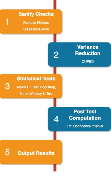
The series, spanning three blogs, initiates a comprehensive analysis, delving into specific steps to illuminate the path toward data-driven success — Part 1 sets the stage, Part 2 describes Statistical Tests and post-test computation, while subsequent details unfold in Part 3.
Statistical Tests
Shapiro Wilk test for Normality
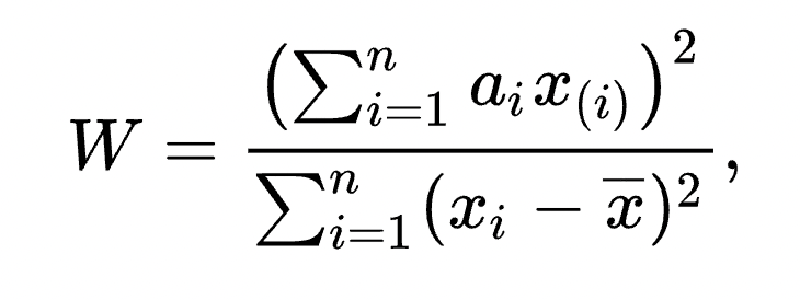
As we embark on the statistical journey, our first stop is the Shapiro-Wilk test, a powerful tool that scrutinizes the normality of continuous, univariate data. This test acts as the litmus test, allowing us to discern whether our sample aligns with the assumptions of a normal distribution.
The Shapiro-Wilk test is a hypothesis test with a null hypothesis that the sample has been generated from a normal distribution. Normality is a crucial assumption for many statistical tests, such as parametric tests like t-tests and ANOVA. Understanding whether your data follows a normal distribution is essential because it allows you to make more accurate inferences and choose appropriate statistical methods.
Note: Normality is a crucial assumption for many statistical tests, such as parametric tests like t-tests. In cases where data follows Normal distribution we use the T-test else we use Non-Parametric tests like the Mann-Whitney U Test.
Welch T Test
Moving into parametric terrain, the Welch T-test takes centre stage. The T-test is a parametric test of difference, meaning that it makes the same assumptions about your data as other parametric tests. The t-test assumes your data:
- are independent — no member of a group should be exposed to both treatment
- are (approximately) normally distributed
- have a similar amount of variance within each group being compared (a.k.a. homogeneity of variance)
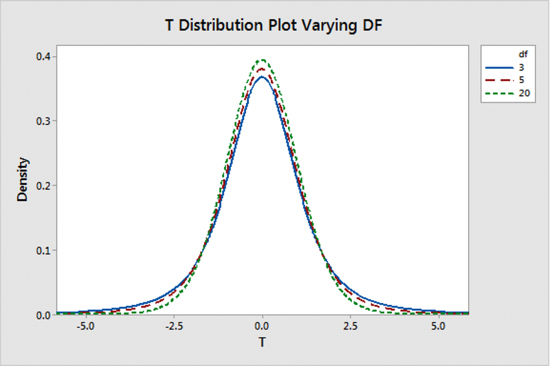
T Statistics
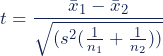
A t-test can only be used when comparing the means of two groups (a.k.a. pairwise comparison). If you want to compare more than two groups, or if you want to do multiple pairwise comparisons, use an ANOVA test.
- For a 1-sample T-test, DF=N-1 because we’re estimating 1 parameter.
- For a 2-sample T-test, DF=N-2 because we’re estimating 2 parameters.
Mann-Whitney U Test
Venturing into the non-parametric realm, we encounter the Mann-Whitney U Test. Also known as the Wilcoxon Rank Sum Test, this method offers a robust alternative for comparing two samples. It is a non-parametric statistical test used to compare two samples or groups.
Steps:
- Assign ranks to the values from the full sample
2. The corresponding Mann–Whitney U statistic is defined as the smaller of:

with R1 & R2 being the sum of the ranks in groups 1 and 2, respectively.
3. Reject H0 if U<= Reference value
Bootstrap Test
The bootstrap method emerges as a saviour for small sample sizes. By oversampling data samples and constructing a histogram of mean values, it presents an efficient and cost-effective approach to hypothesis testing.
If we have a small sample, the mean may be impacted by random effects. So one alternate solution is to repeat the experiment multiple times & create a histogram of the mean values. We can use the histogram to get the probability that mean = 0.
However, repeating the experiment a bunch of times is expensive & time-consuming. Hence instead of replicating the experiment — we can use the Bootstrap Test for the test.
We sample datasets from the original data with replacements and use the mean values to create a histogram of the mean.
Using Bootstrapping to calculate P values
- Shift the raw data so that the mean = 0
- Use bootstrapping to create a histogram of means around 0
- Use the histogram to test the hypothesis that the intervention made 0 difference
MultiLevel Models
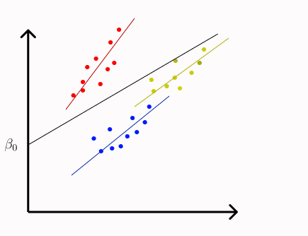
The statistical odyssey continues as we delve into multilevel modelling. Multilevel modelling (also known as hierarchical linear modelling or mixed-effects modelling) is a statistical technique used to analyze data with a hierarchical or nested structure. It accounts for the fact that data points are grouped or clustered within multiple levels, such as individuals within schools, patients within hospitals, or repeated measures within subjects. These models introduce variability in intercept and slope terms, enriching our understanding of complex datasets.
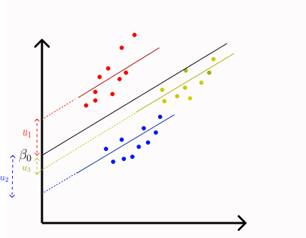
Random Intercept Model
In a random intercept model, the intercept term is allowed to vary across the clusters. As the name suggests we will introduce a random variable for the intercept term.
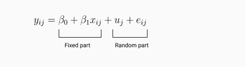
where uj ~ N(0,sigma u2) and eij ~ N(0, sigma e2)
Random Coefficient Model
In a random coefficient model, we allow the slope to vary across the groups. In some cases, random intercept alone may not be sufficient to explain variability across the groups. So, a random slope model is needed where each group will have different slopes along with different intercepts.

import statsmodels.api as sm
import statsmodels.formula.api as smf

data = sm.datasets.get_rdataset("dietox", "geepack").data
md = smf.mixedlm("Weight ~ Time", data, groups=data["Pig"])
mdf = md.fit()
print(mdf.summary())

"""
         Mixed Linear Model Regression Results
========================================================
Model:            MixedLM Dependent Variable: Weight
No. Observations: 861     Method:             REML
No. Groups:       72      Scale:              11.3669
Min. group size:  11      Log-Likelihood:     -2404.7753
Max. group size:  12      Converged:          Yes
Mean group size:  12.0
--------------------------------------------------------
             Coef.  Std.Err.    z    P>|z| [0.025 0.975]
--------------------------------------------------------
Intercept    15.724    0.788  19.952 0.000 14.179 17.268
Time          6.943    0.033 207.939 0.000  6.877  7.008
Group Var    40.394    2.149
========================================================
"""
Post Test Computations
As we traverse the terrain of A/B testing, our journey extends beyond statistical tests to the realm of post-test computations — a phase where the true depth of insights comes to light.
In this section, we unravel the significance of metrics like “Lift,” explore the intricacies of Sample Size Calculations through Power Analysis, and venture into the realm of Confidence Intervals. These post-test computations not only fortify the statistical foundations laid in earlier phases but also empower decision-makers with a nuanced understanding of outcomes.
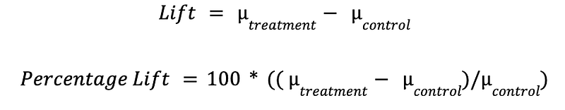
Lift
Transitioning from statistical tests, we delve into post-test computations, commencing with the concept of “Lift.” This metric, the mean average difference between variants, emerges as a pivotal gauge, particularly in the context of A/A tests. It should be close to 0 in the case of the A/A test.
The mean of variants is used to calculate the lift using the following formula.
Sample size calculations (Power Analysis)
Avoiding the pitfalls of P-hacking, power analysis becomes our guide. We do the power analysis to avoid P hacking by determining the required sample size for the experiment.
A power analysis determines what sample size will ensure a high probability that we correctly reject the Null Hypothesis that there is no difference between two groups.
Power is affected by two main factors:
- Overlap between the distributions
Effect size = (Estimated difference between the mean) / (Pooled estimated Standard Deviation)
2. Sample size
Using Effect size, Alpha & 1-Beta, calculate the required sample size using the “Statistics Power Calculator”
Confidence Interval
A confidence interval is a statistical concept that provides a range of values within which we can reasonably estimate the true population parameter to lie. It quantifies the uncertainty associated with a sample statistic and is a crucial tool in inferential statistics.
To calculate a confidence interval of a mean using the critical value of t, we follow these four steps:
- Choose the significance level based on your desired confidence level. The most common confidence level is 95%, which corresponds to α = .05 in the two-tailed t table.
2. Find the critical value of t in the two-tailed t table.
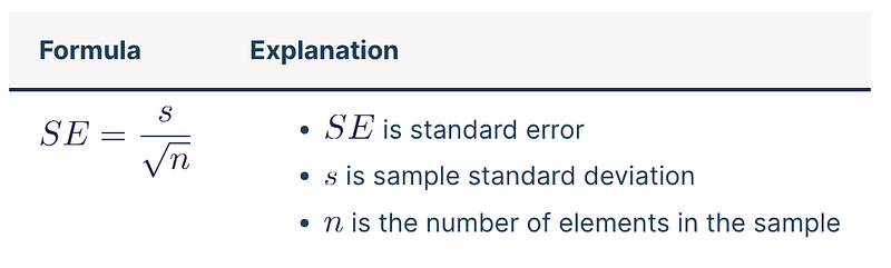
3. Multiply the critical value of t by the Standard error of mean (= standard deviation /√number of observations).
4. Add this value to the mean to calculate the upper limit of the confidence interval, and subtract this value from the mean to calculate the lower limit.
As we wrap up the second instalment of our series, we’ve thoroughly explored the realm of statistical tests and post-test computations, deciphering the complexities of the analysis. The tools and insights unveiled in this section serve as a robust foundation, setting the stage for a deeper understanding of experimental outcomes.
Now, we look ahead to Part 3 — a segment that will provide additional layers of information within our experiment analysis. Beyond statistical tests, we will navigate through other pivotal factors that contribute to the holistic understanding of experimental data.
To continue exploring the successive components of this series, please refer to Part 3 of the blog.
References:
- https://en.wikipedia.org/wiki/Shapiro%E2%80%93Wilk_test
- https://library.virginia.edu/data/articles/understanding-q-q-plots
- https://www.statology.org/welchs-t-test/
- https://en.wikipedia.org/wiki/Mann%E2%80%93Whitney_U_test
- https://www.youtube.com/watch?v=Xz0x-8-cgaQ
- https://en.wikipedia.org/wiki/Random_effects_model
- https://www.statskingdom.com/sample_size_t_z.html
If you have read so far, a big thank you for reading! I hope you find this article to be helpful. If you’d like, add me on LinkedIn!
Good luck this week, Pratyush