Summary

This article delves into the application of Decision Trees and Random Forests for classification and regression tasks, emphasizing the robustness and simplicity of Random Forests as a learning model that mitigates overfitting.

Abstract

The article provides an in-depth exploration of Bootstrap Aggregation (bagging) and its role in enhancing the stability and performance of learning models, particularly Random Forests. It explains how bagging reduces variance and overfitting by creating multiple subsets of the original dataset and aggregating the outputs of individual learning models. The concept of Random Forests is introduced as an ensemble of Decision Trees, each trained on bootstrap samples with a random subset of features, leading to improved variable selection and model performance. The article also discusses practical aspects such as choosing the number of trees and the importance of feature selection in Random Forest models, using scikit-learn's RandomForestClassifier as an example. It concludes with the significance of benchmarking simpler models like Random Forests against more complex ones and encourages readers to engage with the provided Jupyter Notebook for a hands-on understanding of the concepts discussed.

Opinions

The author posits that Random Forests, through their combination of Decision Trees and bagging, offer a powerful yet straightforward approach to supervised learning problems.
It is suggested that the increase in bias introduced by bagging is typically outweighed by the reduction in variance, making it a favorable trade-off in practical applications.
The article conveys that Random Forests are not only efficient in terms of computational speed but also versatile in their ability to perform classification, regression, and feature selection.
The author emphasizes the importance of understanding the bias-variance trade-off and selecting the appropriate number of trees and features for optimal model performance.
There is an opinion that simpler models like Random Forests should be benchmarked against more sophisticated models to ensure the best approach is taken for a given problem.
The author encourages interactive learning by providing a Jupyter Notebook for readers to explore the feature importance and F1 score diagnostics, demonstrating a hands-on approach to learning.

Decision Trees and Random Forests for Classification and Regression pt.2

Forest from the trees, mountains from the dust.

Highlights:

In this article, we will take a look at the following:

Bootstrap aggregation for robust learning
Random forests for variable selection
Random forests for fast and robust regression, classification and feature selection analysis

Link to part 1 here.

Link to Neptune.ai article on where Random Forest algorithms can fail: https://neptune.ai/blog/random-forest-regression-when-does-it-fail-and-why

Links to my other articles:

Introduction:

In my last article we covered Decision Trees and how they can be used for classification and regression. This article, we will continue where we left off and introduce ensemble Decision Tree models or so-called Random Forests. We’ll see how the combination of the advantages of Decision Trees combined with Bootstrap aggregation make Random Forests a remarkably robust yet simple learning model less prone to overfitting vs single Decision Trees for supervised learning problems. To get a sense of the power of Random Forests, here’s using them to identify spy-planes being flown by the US Government from publicly available flight path data.

Bootstrap Aggregation:

Bootstrap Aggregation, or bagging is a powerful technique that reduces model variances (overfitting) and improves the outcome of learning on limited sample (i.e. small number of observations) or unstable datasets. Bagging works by taking the original dataset and creating M subsets each with n samples per subset. The n individual samples are uniformly sampled with replacement from the original dataset. The diagram below illustrates this.

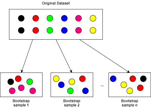
In the diagram above, the labels corresponding to each data point are preserved. In other words, each data tuple (X,Y)ᵢ is sampled and subsetted where each Xᵢ is a vector of inputs and Yᵢ is a vector of responses. Theoretically, as the number of bootstrap samples M approaches infinity, bagging is shown to converge to the mean of some non-bagged function estimator utilizing all possible samples from the original dataset (intuitively, this makes sense). In the context of stochastic gradient learning, in for example neural networks or logistic regression, learning from multiple (repeated) data samples in random order tends to increase learning performance, as the gradient estimate tends to be ‘jostled around’ more with the hopes of overcoming local extrema. As well, an interesting result shown in Bühlmann’s article indicates that bagging tends to add bias to the bagged estimator, with the tradeoff of reducing variance. In most practical applications, this increase in bias is small compared to the reduction in variance. In general, the bias-variance trade-off is a very important aspect of statistical learning and in picking your supervised learning models, something that the adept data magician should be well aware of.

Next, k individual learning models (called an ensemble) are created for each M bootstrap sample. The outputs of each individual learning model are then aggregated or averaged in some way, such as voting or simple means averaging. This is illustrated in the figure below.

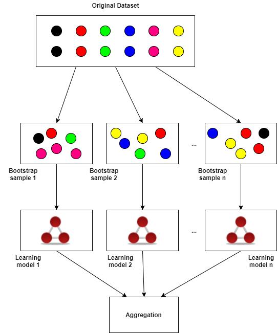
In general, bagging with ensemble models is a robust method for reducing the variance and overfitting of your learning models by utilizing bootstrap samples and aggregating the output (mean, median, other more complicated methods) of the learning ensembles. Bagging and ensembles are general and can be applied to any supervised model from neural networks to SVMs to decision trees, as well as unsupervised clustering models (to be covered in another article). In practice, M is chosen to be at least 50 and n is 80% of the size of the original dataset.

Random Forests:

Random Forests are an ensemble of k untrained Decision Trees (trees with only a root node) with M bootstrap samples (k and M do not have to be the same) trained using a variant of the random subspace method or feature bagging method. Note the method of training random forests is not quite as straightforward as applying bagging to a bunch of individual decision trees and then simply aggregating the output. The procedure for training a random forest is as follows:

At the current node, randomly select p features from available features D. The number of features p is usually much smaller than the total number of features D.
Compute the best split point for tree k using the specified splitting metric (Gini Impurity, Information Gain, etc.) and split the current node into daughter nodes and reduce the number of features D from this node on.
Repeat steps 1 to 2 until either a maximum tree depth l has been reached or the splitting metric reaches some extrema.
Repeat steps 1 to 3 for each tree k in the forest.
Vote or aggregate on the output of each tree in the forest.

Compared with single decision trees, random forests split by selecting multiple feature variables instead of single features variables at each split point. Intuitively, the variable selection properties of decision trees can be drastically improved using this feature bagging procedure. Typically, the number of trees k is large, on the order of hundreds to thousands for large datasets with many features.

Variable Selection:

Variable selection with Random Forests is quite simple. Using scikit-learn’s RandomForestClassifier, let’s load up our favorite dataset (the one with the fancy wines) and take a look at what our random forest classifier thinks are the most important features for wine classification. Scroll through the Jupyter Notebook to see the feature information plot and the average F1 score as a function of the number of features (you should probably download the Jupyter Notebook file/gist from my github to see the plots better).

Interestingly, the proline content still comes out on top as the feature with the most information when n_trees = 1000. Training with 1000 trees takes a few seconds on my Core i7 laptop, which is much faster than most deep neural net models. With lesser trees, color_intensity tends to come out on top. When n_trees = 1000, color_intensity can still be quite close to proline content. In general you should do a sweep of the hyperparameter n_trees and assess the diagnostic plots to get a good idea of the dataset and what features are important. Once you have plotted the relative information/importance plots of each feature, features above a certain threshold can be used in another learning model such as deep neural net, and features below the threshold can be ignored. The F1 score sweep across the number of features should be done on a very constrained ensemble model with a limitingly small number of learners. The F1 sweep plot in the notebook shows the effect of adding features or variables to a model, namely the effect of adding more input features on classification accuracy (note F1 scores and AUROCs are only defined for classification problems, regression problems require a different error measure such as Mean Square Error).

In Summary:

Random forests can be used for robust classification, regression and feature selection analysis. Hopefully you can see that there still a few tricks you need to apply first before you can expect decent results.

With respect to supervised learning problems, it’s always a good idea to benchmark your simpler models such as Random Forests versus complicated deep Neural Networks or Probabilistic Models. If you have any questions about running the code, or about the mysteries of life in general, please don’t hesitate to ask me.