Decision Trees and Random Forests for Classification and Regression pt.1

Highlights:

Want to use something more interpertable, something that trains faster and performs pretty much just as well as the old Logistic Regression or even Neural Networks? You should consider Decision Trees for classification and regression. Part 2 on Random Forests here.

Much faster to train versus simple neural networks for comparable performance (The time complexity of decision trees is a function of [number of features, number of rows in dataset], whereas for neural networks it is a function of [number of features, number of rows in dataset, number of hidden layers, number of nodes in each hidden layer])
Easily interpretable, suitable for variable selection
Fairly robust on smaller datasets
Decision Trees and Decision Tree Learning are simple to understand

Links to my other articles:

Introduction:

Decision Trees and their extension Random Forests are robust and easy-to-interpret machine learning algorithms for Classification and Regression tasks. Decision Trees and Decision Tree Learning together comprise a simple and fast way of learning a function that maps data x to outputs y, where x can be a mix of categorical and numeric variables and y can be categorical for classification, or numeric for regression. Methods such as SVMs, Logistic Regression and Deep Neural Nets pretty much do the same thing. However despite their power against larger and more complex datasets, they are extremely hard to interpret and neural nets can take many iterations and hyperparameter adjustments before a good result is had. As well, one of the biggest advantages of using Decision Trees and Random Forests is the ease in which we can see what features or variables contribute to the classification or regression and their relative importance based on their location depthwise in the tree.

We’ll look at decision trees in this article and compare their classification performance using information derived from the Receiver Operating Characteristic (ROC) against logistic regression and a simple neural net.

Decision Trees:

A Decision Tree is a tree (and a type of directed, acyclic graph) in which the nodes represent decisions (a square box), random transitions (a circular box) or terminal nodes, and the edges or branches are binary (yes/no, true/false) representing possible paths from one node to another. The specific type of decision tree used for machine learning contains no random transitions. To use a decision tree for classification or regression, one grabs a row of data or a set of features and starts at the root, and then through each subsequent decision node to the terminal node. The process is very intuitive and easy to interpret, which allows trained decision trees to be used for variable selection or more generally, feature engineering. To illustrate this, suppose you wanted to buy a new car to drive up a random dirt road into a random forest. You have a dataset of different cars with three features: Car Drive Type (Categorical), Displacement (Numeric) and Clearance (Numeric). An example of a learned decision tree to help you make your decision is below:

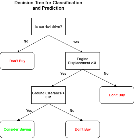
I like to go off-roading when I’m not making machines learn.

The root or topmost node of the tree (and there is only one root) is the decision node that splits the dataset using a variable or feature that results in the the best splitting metric evaluated for each subset or class in the dataset that results from the split. The decision tree learns by recursively splitting the dataset from the root onwards (in a greedy, node by node manner) according to the splitting metric at each decision node. The terminal nodes are reached when the splitting metric is at a global extremum. Popular splitting metrics include the minimizing the Gini Impurity (used by CART) or maximizing the Information Gain (used by ID3, C4.5).

Example:

Now that we have seen how decision tree training works, let’s use the scikit-learn package (scikit-learn contains many nice data processing, dimensionality reduction, clustering and shallow machine learning tools) and implement a simple decision tree for classification on the Wine Dataset (13 features/variables with 3 classes), and then visualize the learned tree with Graphviz.

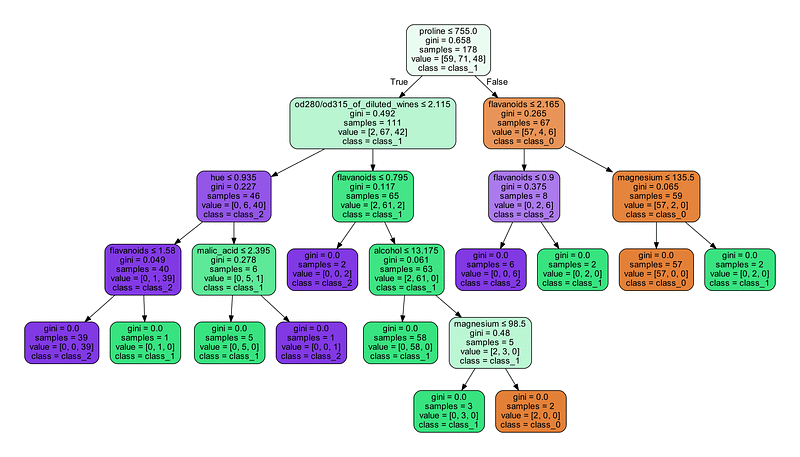
No need to waste money on wine tasting courses.

Right away, from the learned decision tree we can see that the feature proline (proline content in the wine) is the root node with the highest Gini Impurity value of 0.658, and this means that all three wine classes have this as their base separation. This also means that in principle, if we used only one feature in a predictive model, the proline content will allow us to predict correctly to a maximum 1-0.658 = 0.342 = 34.2% of the time, assuming that the original learned decision tree predicts perfectly. Then, from the root we see that the classes split off further with the od280/od315_of_dilute_wines feature and the flavinoid feature. We can also see that a majority of the class_1 wine (81.7%) have an alcohol content ≤ 13.175 and a flavinoid content ≤ 0.795. Also, recall that there are 13 features in the original dataset, but the decision tree picked only a subset of 7 features for the classification.

We can use this information to select which features/variables in a general dataset are important (in cases where there may be non-useful, redundant or noisy features) for a more advanced model such a deep neural net. We’ll see how to do this with more robust random forests in part 2. The learned decision tree can be used to predict data using a simple function call on a row of input data. A regression tree for predicting numerical output values from input features can be created very easily as well: check out this scikit-learn tutorial.

Performance:

The Receiver Operating Characteristic (ROC) is a plot that can be used to determine the performance and robustness of a binary or multi-class classifier. The x-axis is the false positive rate (FPR) and the y-axis is the true positive rate (TPR). The ROC plot gives information about the about true postive/negative rate and false positive/negative rate and something called the C-statistic or area under ROC curve (AUROC) for each class predicted by the classifier (there is one ROC for each class predicted by the classifier). The AUROC is defined as the probability that a randomly selected positive sample will have a higher prediction value than a randomly selected negative sample. A quote from this article on the subject:

“Assuming that one is not interested in a specific trade-off between true positive rate and false positive rate (that is, a particular point on the ROC curve), the AUC [AUROC] is useful in that it aggregates performance across the entire range of trade-offs. Interpretation of the AUC is easy: the higher the AUC, the better, with 0.50 indicating random performance and 1.00 denoting perfect performance.”

The AUROCs for different classifiers can be compared against each other. Alternatives to this metric include using the scikit-learn confusion matrix calculator for the prediction results and using the resultant matrix to derive basic positive/negative accuracy, F1-scores, etc.

{0: 0.98076923076923084, 1: 0.97499999999999998, 2: 1.0, 'micro': 0.97916666666666685}

The above output is the AUROC for each class predicted by the decision tree. The compare, in scikit-learn we re-run the same dataset with 20% test set on a logistic regression model and a shallow MLP neural net model. The logistic regression model’s performance (with all default parameters) is below:

{0: 0.96153846153846156, 1: 0.94999999999999996, 2: 1.0, 'micro': 0.95833333333333326}

And for the shallow MLP net: hidden layers = 2, nodes per layer = 25, optimizer = adam, activation = logistic, iterations = 50000:

{0: 1.0, 1: 1.0, 2: 1.0, 'micro': 1.0}

We can see that the decision tree outperforms logistic regression, and although the Neural Net beats it, it is still much faster to train and has the advantage of interpretability.

What’s Next:

Decision Trees should always be in the toolkit of the adept Data Scientist and Machine Learning Engineer. For a more thorough user guide/manual of how to use decision trees in scikit-learm, refer to http://scikit-learn.org/stable/modules/tree.html#decision-trees.

However, despite the ease of use and apparent power of decision trees, their reliance on a greedy strategy for learning may cause the tree to split the wrong features at each node or cause the tree to overfit. Stay tuned, in the next article I will be demonstrating ensemble decision trees, or so-called Random Forests and Bootstrap Aggregation which when used together drastically increase predictive power and robustness for larger and more complicated datasets. As well we’ll see how we can use random forests for robust Variable Selection.