Black Swans and Hockey Riots: Extreme Value Analysis and Generalized Extreme Value Distributions

In this article, we’ll look at:

• A brief introduction to the theory of Extreme Value Analysis (EVA) and the Generalized Extreme Value (GEV) distribution for estimating the probability of outlier events
• Applying GEV fitting and analysis to a practical time series problem using the block maxima method in R Studio
• Predicting the probability of another hockey riot in Vancouver.

Links to my other articles:

1. Random forests
2. Softmax classification
3. Climate analysis

Introduction:

Nassim Taleb’s book The Black Swan: The Impact of the Highly Improbable (2007) introduced to the general public what Actuaries, Engineers and Options Traders have secretly known about and struggled with for quite a long time. Taleb’s book talks about how outlier events with extreme impacts called ‘black swans’ actually occur more often than people think, and by corollary how people fail to adequately design against or prepare for these events. For example, natural disasters such as the 9.1 magnitude 2011 Tōhoku earthquake (which caused the Fukushima nuclear meltdown) and man-made disasters such as the 2008 Global Financial Crisis qualify as black swans.

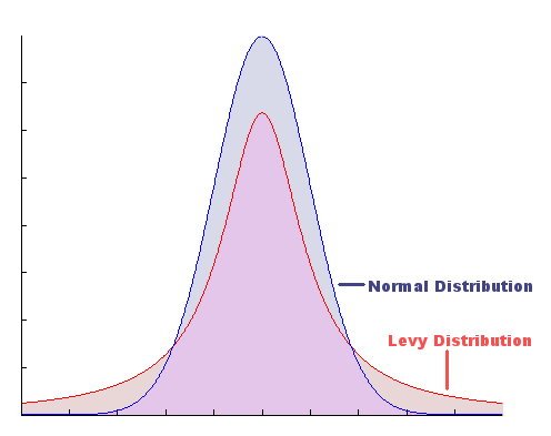
Part of the reason why professionals who employ statistics in their work to make decisions such as Hydrologists, Quants and Data Scientists (haha…right?) historically underestimate the probability of these black swans is because they predominately rely on Gaussian models, and unfortunately the real world is not really Gaussian. Pioneering work by mathematicians such as Beniot Madelbrot showed that random variables observed from real-world processes, such as stock returns or daily river levels follow ‘fat-tailed’ distributions that are quite different from Gaussians. These fat tailed distributions have high probability densities in their tails, implying that outliers are more likely than Gaussian. According to Wikipedia they have higher skewness and kurtosis vs. Gaussian or Exponential distributions. An example of a Gaussian (Normal) distribution and a fat-tailed Levy distribution is shown below.

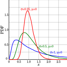
A log-normal distribution for certain parameters is an example of a two tailed fat tail distribution that can be considered one sided.

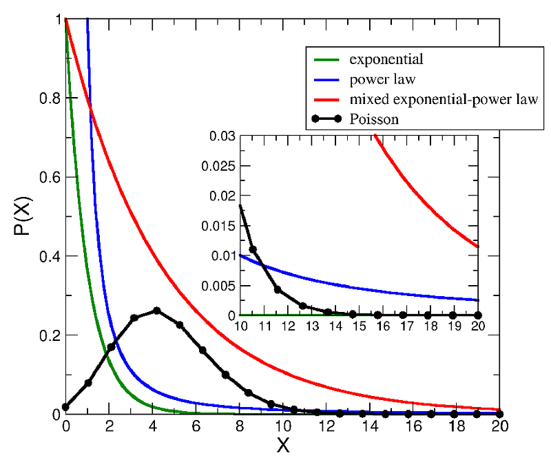
And examples of ‘exponential-shaped’ fat-tailed distributions which are strictly one sided.

While the junior Engineer may employ some sort of ‘trial and error’ method to fit all possible fat-tailed distributions to his empirically observed data, the far more elegant and mathematically rigorous™ way to quantify the density in these fat-tails — and by corollary to quantify the probability of outliers which depending on the problem you’re trying to solve may or may not have catastrophic implications — is by using Extreme Value Analysis (EVA).

The Theory of Extreme Values:

Sometime in the early 60’s came along a remarkable theorem called the Fisher–Tippett–Gnedenko theorem which is an analog of the Central Limit Theorem in probability theory but applied to ‘sample extrema’ instead of sample means. Basically the FTG theorem states that for an iid sequence of random variables (for example a time-series segregated into blocks), we can construct another sequence called M consisting of the maxima of each random variable (or minima of each), and if the (normalized) distribution of M converges asymptotically (sample size n tends to infinity) it must converge to one of three distributions called Gumbel, Fréchet and (reverse) Weibull. For an outline of the proof of the FTG theorem see here.

For convenience, the three EV distributions mentioned above have been combined into a single Generalized Extreme Value (GEV) distribution.

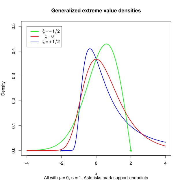
The GEV distribution is a three-parameter distribution and more details regarding the parameters can be found here. In brief, the three parameters are μ, σ and ξ. The parameter μ determines the location or mean of the GEV, σ affects the skew and kurtosis, and ξ affects the general shape of the distribution (which also affects skew and kurtosis). In the above plot the support for the GEV (the x axis) represents the magnitude of the extreme values themselves.

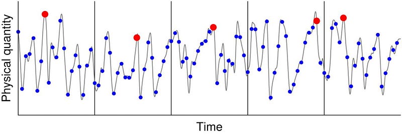
The particular application of FTG and EVA we will talk about in this article is the ‘block maxima’ method. The block maxima method directly extends the FTG theorem given above and the assumption is that each block forms a random iid sample from which an extreme value distribution can be fitted. So in other words, we will fit a GEV distribution to the extrema sampled from each block. There is another method called Peak over Threshold (PoT) which assumes a different distribution (Generalized Pareto or GP) and a different way to sample the extreme values. PoT will be covered in another article if I feel like it.

Once we have partitioned the time series into blocks of suitable length, the familiar Maximum Likelihood Estimation (MLE) method is used to actually fit the GEV parameters to the block maxima samples. Alternative methods such as the method of L-moments exist and may give a better fit in some cases. Fortunately the package we will use to do the GEV fit has both MLE and L-moments methods.

Time Series EVA on Daily Reported Crimes:

We will now apply block maxima EVA to predict the probability of monthly crime spikes in Vancouver BC and the expected period of months before a certain monthly reported crime count threshold is exceeded. This dataset is a good candidate for EVA because of the presence of an extreme outlier event in 2011 which caused an all-time-high spike in the reported crime counts dataset. Interestingly enough this was not the first hockey riot in Vancouver.

So let’s go and fetch the Vancouver Crimes dataset from kaggle: https://www.kaggle.com/wosaku/crime-in-vancouver. Props to Willan Osaku for the data wrangling as done in his kernel here: https://www.kaggle.com/wosaku/eda-of-crime-in-vancouver-2003-2017. The dataset contains reports of property crimes and crimes committed against people from Jan 1 2003 to Jul 15 2017. We will set the block maxima size to 30 days regardless of the number of days in calendar months. Edit: for your convenience, all data sets (the original and the daily aggregate) are available here: https://github.com/hhl60492/blog

For this analysis we will be using a combination of python and R. Python for the data wrangling and R for the actual GEV fitting (at this point Python lacks the high quality EVA packages that R has). For the python script, basically we aggregate the reported number of crimes by day, plot it and dump that data series to a csv with the dates.

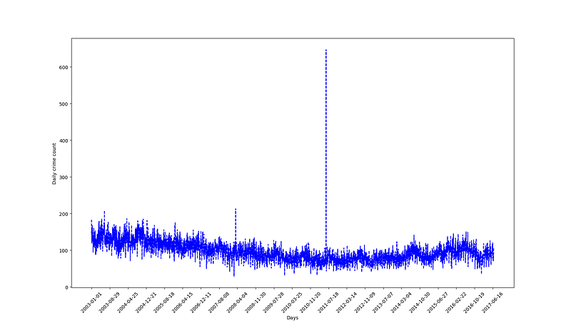
In the above daily crime reports time series, we have a median of 95 crimes per day, with min = 29 and max = 647, with stddev = 26.

Next, we are going to download and install the package ‘extRemes’ package in RStudio. Then EVA is as straightforward as loading the package, aggregating the data and doing the necessary fits. However, interpreting the ‘return ’ of the GEV is where the meat and potatoes are and we’ll get to that in a bit.

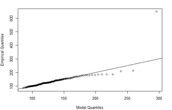
Note the way the block maxima was aggregated was on a 30-day interval regardless of calendar months (aggregates on calendar months giving variable block maxima sizes does not really affect our fit). Now, the diagnostic plots given by

plot(fit_mle)

such as the Emperical vs Model Q-Q Plot gives an indication of how good the fit is (the more dots that fall on the line the better). We see evidence of an extreme outlier that was too extreme for even our GEV.

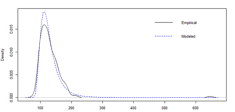
And below is what our fitted GEV actually looks like compared to the empirical block max sample distribution/histogram.

fevd(x = as.vector(month_bm$month_max), type = "GEV", method = "Lmoments", 
    period.basis = "month")
[1] "GEV  Fitted to  as.vector(month_bm$month_max)  using L-moments estimation."
   location       scale       shape 
114.0563798  19.6206000   0.2034706

There really isn’t too much of a difference in fit between the MLE and L-moment GEV models, so let’s just pick the L-moment model and print out the return levels.

fevd(x = as.vector(month_bm$month_max), type = "GEV", method = "Lmoments", 
    period.basis = "month")
get(paste("return.level.fevd.", newcl, sep = ""))(x = x, return.period = return.period, 
    conf = 0.05)

GEV model fitted to  as.vector(month_bm$month_max)  
Data are assumed to be  stationary 
[1] "Return Levels for period units in months"
  3-month level   6-month level  12-month level  24-month level  48-month level 120-month level 
       133.4993        153.9620        176.1072        200.9296        229.1534        272.8342

The results from “Return Levels for period units in months” on are the return period and corresponding return level on the line below it. The return value is defined as a value that is expected to be equaled or exceeded on average once every return period. The return period T of a particular event is the inverse of the probability that the event will be exceeded in any given block maxima time unit. Note T is always a multiple of our base block maxima time unit (in our case 1 month = 30 days) and is related to the threshold exceedance probability p by T = 1/p.

So what this all means is that for the foreseeable future (assuming the distribution does not change, i.e. stationarity; also one should refit and revise predictions after every block max period has elapsed) from the first return period we can expect on average one instance of seeing more than 133.5 crimes reported per day in a 3-month period.

Conversely if we wanted to see how likely it is for one of next month’s daily crime reports to exceed 133.5, it would be 1/(3 months) or 33.3% (again, under strict stationarity assumptions). Looking at the largest return period, our interpretation would be that there is likely to be a day exceeding 272.8 crime reports in the next 120 months (10 years) or conversely the probability of seeing a day exceeding 272.8 crime reports in the next 30 days is 1/120 = 0.83%.

As an fun exercise let’s try to predict the probability of another hockey riot in Vancouver. The empirical data (with a terrible sample size of n=2) gives us 2 hockey riots in 17 years. Thus the yearly rate of hockey riots according to the empirical data is 2/17 or 11.76%. You can run a block max and GEV fit on hockey riot counts distributed across years or decades but fitting on only 2 empirical data points is terrible idea, only slightly better than participating in a hockey riot yourself. So let’s find a better way of estimating the probability of another hockey riot. We know that during hockey riots many crimes reports will get submitted to the police. Thus we can use the daily reported crime counts as a proxy for the riots. Now there are no data points going back to 1994 regarding how many crimes were reported on the day of the riot, but this CBC article states that there were 150 arrests made in connection to the riot. So for that day of the riot in 1994, let’s assume a base crime report count of 96 (the median of our 2003–2017) and a conversion factor of 1.5 for arrests to reported crime numbers, as the rioters may have created more than one crime report per arrest or conversely some rioters got away and were not arrested after a crime report was created. So for the day of the 1994 riot we have perhaps 96 + 1.5 * 150 = 321 crimes reported. Then the average number of crimes reported between both riots is (647+321) / 2 = 484.

Next, we will work backwards and modify the return period in our call to the return.level() function and use trial and error to find the period that gives us a return level close to 484 in our GEV fitted to the 2003 to 2017 dataset.

return.level(fit_lmom, conf = 0.05, return.period= c(3,6,12,24,48,120*20))

Gives us return levels of

3-month level    6-month level   12-month level   24-month level   48-month level 2400-month level 
        133.4993         153.9620         176.1072         200.9296         229.1534         487.4839

Bingo. So the chance of one hockey riot in the next month based on this analysis is approximately 1/2400 or 0.042%. Assuming the GEV remained stationary and that hockey riots occur independently of one and another, we will have on average 1 hockey riot or other mass crime incident where the daily crime count exceed 484 reports in the next 200 years. Disclaimer: this analysis is for educational purposes only. It is not meant to inform any decision making on part of any person currently residing in, moving into or out of Vancouver, affected businesses, the Municipal Government, Provincial Government, the VPD, nor the RCMP.

Conclusion:

In practice, it is wise to refit the GEV and revise the updates after every single block maxima period has elapsed. Moreso, standard time series practices such as de-trending and seasonality removal may help to give the GEV a better fit. Recently, non-stationary EVA methods have been developed, but the theoretical framework for non-stationary GEV models has not been well established. If you are interested, checkout NEVA (Matlab) and GEV-CDN (R). However in general the limitation of EVA must be acknowledged. The EVA distributions fit only what is observed from a univariate time series, and makes no assumptions regarding external factors that affect the system under study. Even in the case of non-stationary EVA, the non-stationarities are chosen a-priori to be some simple continuous functions and are still mostly agnostic to external factors. Good luck doing your own Extreme Value Analysis, and be sure to check off with your senior Statistician specializing in Extreme Value Theory before making any decision based on your predictions!