Applied Reinforcement Learning V: Normalized Advantage Function (NAF) for Continuous Control

Introduction and explanation of the NAF algorithm, widely used in continuous control tasks

If you want to read this article without a Premium Medium account, you can do it from this friend link :) https://readmedium.com/applied-reinforcement-learning-v-normalized-advantage-function-naf-for-continuous-control-62ad143d3095?sk=29dcca538748f7b05c18b6d1c092a8cc

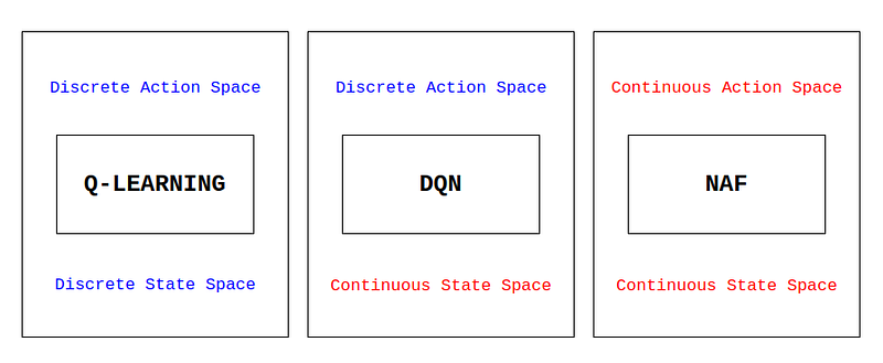
Previous articles in this series have introduced and explained two Reinforcement Learning algorithms that have been widely used since their inception: Q-Learning and DQN.

Q-Learning stores the Q-Values in an action-state matrix, such that to obtain the action a with the largest Q-Value in state s, the largest element of the Q-Value matrix for row s must be found, which makes its application to continuous state or action spaces impossible since the Q-Value matrix would be infinite.

On the other hand, DQN partially solves this problem by making use of a neural network to obtain the Q-Values associated to a state s, such that the output of the neural network are the Q-Values for each possible action of the agent (the equivalent to a row in the action-state matrix of Q-Learning). This algorithm allows training in environments with a continuous state space, but it is still impossible to train in an environment with a continuous action space, since the output of the neural network (which has as many elements as possible actions) would have an infinite length.

The NAF algorithm introduced by Shixiang Gu et al. in [1], unlike Q-Learning or DQN, allows training in continuous state and action space environments, adding a great deal of versatility in terms of possible applications. Reinforcement learning algorithms for continuous environments such as NAF are commonly used in the field of control, especially in robotics, because they are able to train in environments that more closely represent reality.

Introductory Concepts

Advantage Function

State-Value Function V and Action-Value Function (Q-Function) Q, both explained in the first article of this series, determine the benefit of being in a state while following a certain policy and the benefit of taking an action from a given state while following certain policy, respectively. Both functions, as well as the definition of V with respect to Q, can be seen below.

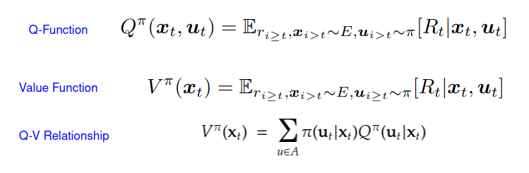
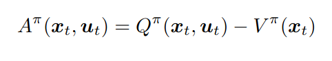
Since Q returns the benefit of taking a certain action in a state, while V returns the benefit of being in a state, the difference of both returns information about how advantageous it is to take a certain action in a state with respect to the rest of actions, or the extra reward that the agent will receive by taking that action with respect to the rest of actions. This difference is called Advantage Function, and its equation is shown below.

Ornstein-Uhlenbech Noise Process (OU)

As seen in previous articles, in Reinforcement Learning algorithms for discrete environments such as Q-Learning or DQN, exploration is performed by randomly choosing an action and ignoring the optimal policy, as is the case for epsilon greedy policy. In continuous environments, however, the action is chosen following the optimal policy, and adding noise to this action.

The problem with adding noise to the chosen action is that, if the noise is uncorrelated with the previous noise and has a distribution with zero mean, then the actions will cancel each other out, so that the agent will not be able to maintain a continuous movement to any point but will get stuck and therefore will not be able to explore. The Ornstein-Uhlenbech Noise Process obtains a noise value correlated with the previous noise value, so that the agent can have continuous movements towards some direction, and therefore explore successfully.

More in-depth information about the Ornstein-Uhlenbech Noise Process can be found in [2]

Logic behind the NAF algorithm

The NAF algorithm makes use of a neural network that obtains as separate outputs a value for the State-Value Function V and for the Advantage Function A. The neural network obtains these outputs since, as previously explained, the result of the Action-Value Function Q can be later obtained as the sum of V and A.

Like most Reinforcement Learning algorithms, NAF aims to optimize the Q-Function, but in its application case it is particularly complicated since it uses a neural network as Q-Function estimator. For this reason, the NAF algorithm makes use of a quadratic function for the Advantage Function, whose solution is closed and known, so optimization with respect to the action is easier.

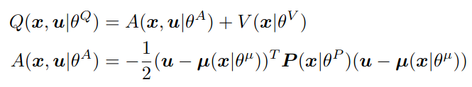
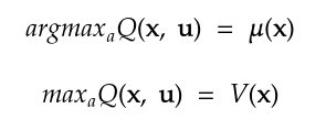
More specifically, the Q-Function will always be quadratic with respect to the action, so that the argmax Q(x, u) for the action is always 𝜇(x|𝜃) [3], as shown in Figure 2. Thanks to this, the problem of not being able to obtain the argmax of the neural network output due to working in a continuous action space, as was the case with DQN, is solved in an analytical way.

By looking at the different components that make up the Q-Function, it can be seen that the neural network will have three different outputs: one to estimate the Value Function, another to obtain the action that maximizes the Q-Function (argmax Q(s, a) or 𝜇(x|𝜃)), and another to calculate the matrix P (see Figure 1):

• The first output of the neural network is the estimate of the State-Value Function. This estimate is then used to obtain the estimate of the Q-Function, as the sum of the State-Value Function and the Advantage Function. This output is represented by V(x|𝜃) in Figure 1.
• The second output of the neural network is 𝜇(x|𝜃), which is the action that maximizes the Q-Function on the given state, or argmax Q(s, a), and therefore acts as the policy to be followed by the agent.
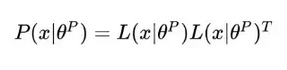
• The third output is used to later form the state-dependent, positive-definite square matrix P(x|𝜃). This linear output of the neural network is used as entry for a lower-triangular matrix L(x|𝜃), whose diagonal terms are exponentiated, and from which the mentioned matrix P(x|𝜃) is constructed, following the following formula.

The second and third outputs of the neural network are used to construct the estimate for the Advantage Function as shown in Figure 1, which is then added to the first output (the State-Value Function estimate V) to obtain the estimate for the Q-Function.

Regarding the rest of the NAF algorithm flow, it includes the same components and steps as the DQN algorithm explained in article Applied Reinforcement Learning III: Deep Q-Networks (DQN). These components in common are the Replay Buffer, the Main Neural Network and the Target Neural Network. As for DQN, the Replay Buffer is used to store experiences to train the main neural network, and the target neural network is used to calculate the target values and compare them with the predictions from the main network, and then perform the backpropagation process.

NAF Algorithm Flow

The flow of the NAF algorithm will be presented following the pseudocode below, extracted from [1]. As mentioned above, the NAF algorithm follows the same steps as the DQN algorithm, except that NAF trains its main neural network differently.

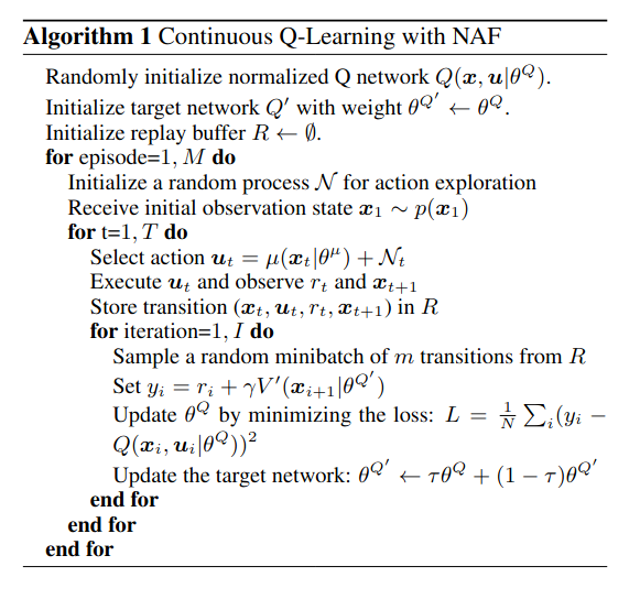
For each timestep in an episode, the agent performs the following steps:

1. From given state, select an action

The action selected is the one that maximises the estimate of the Q-Function, which is given by the term 𝜇(x|𝜃), as shown in Figure 2.

To this selected action the noise extracted from the Ornstein-Uhlenbech noise process (previosuly introduced) is added, in order to enhance the agent’s exploration.

2. Perform action on environment

The action with noise obtained in the previous step is executed by the agent in the environment. After the execution of such an action, the agent receives information about how good the action taken was (via the reward), as well as about the new situation reached in the environment (which is the next state).

3. Store experience in Replay Buffer

The Replay Buffer stores experiences as {s, a, r, s’}, being s and a the current state and action, and r and s’ the reward and new state reached after performing the action from the current state.

The following steps, from 4 to 7, are repeated as many times as stated in the algorithm’s hyperparameter I per timestep, which can be seen in the pseudocode above.

4. Sample a random batch of experiences from Replay Buffer

As explained in the DQN article, a batch of experiences is extracted only when the Replay Buffer has enough data to fill a batch. Once this condition is met, {batch_size} elements are randomly taken from the Replay Buffer, giving the possibility to learn from previous experiences, without the need to have lived them recently.

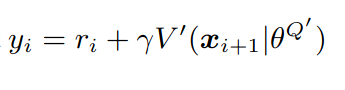
5. Set the target value

The target value is defined as the sum of the reward and the Value function estimate of the Target neural network for the next state multiplied by the discount factor γ, which is an hyperparameter of the algorithm. The formula for the target value is shown below, and it is also available in the pseudocode above.

6. Perform Gradient Descent

Gradient Descent is applied to the loss, which is calculated with the estimate of the Q-Function obtained from the main neural network (predicted value) and the previously calculated target value, following the equation shown below. As can be seen, the loss function used is the MSE, so the loss will be the difference between the Q-Function estimate and the target squared.

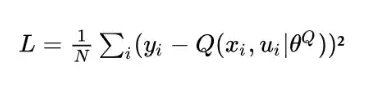
It should be remembered that the estimate of the Q-Function is obtained from the sum of the estimate of the Value Function V(x|𝜃) plus the estimate of the Advantage function A(x, u|𝜃), whose formula is shown in Figure 1.

7. Softly update the Target Neural Network

The weights of the Target neural network are updated with the weights of the Main neural network in a soft manner. This soft updation is performed as a weighted sum of the Main network’s weights and the Targt network’s old weights, as shown in the following equation.

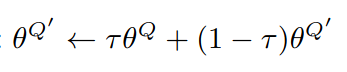
The importance of the weights of each neural network in the weighted sum is given by the hyperparameter τ. If τ is zero, the target network will not update its weights, since it will load its own old weights. If τ is set to 1, the target neural network will be updated by loading the weights of the main network, ignoring the old weights of the target network.

8. Timestep ends — Execute the following timestep

Once the previous steps have been completed, this same process is repeated over and over again until the maximum number of timesteps per episode is reached or until the agent reaches a terminal state. When this happens, it goes to the next episode.

Conclusion

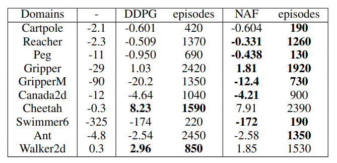
The NAF algorithm achieves really good results in its implementation in continuous environments, so it fulfills its objective satisfactorily. The results of NAF in comparison with the DDPG algorithm [4] are shown below, where it can be seen how it improves considerably on the previous work. In addition, the beauty of the NAF algorithm should be highlighted, as it deals with the limitations of DQN for continuous environments with the cuadratic functions and its easy optimization, a smart and creative solution.

On the other hand, although NAF has shown to be an efficient and useful algorithm, its logic and implementation is not simple, especially when compared to previous algorithms for discrete environments, which makes it hard to use.

REFERENCES

[1] GU, Shixiang, et al. Continuous deep q-learning with model-based acceleration. En International conference on machine learning. PMLR, 2016. p. 2829–2838

[2] Ornstein-Uhlenbech Process https://en.wikipedia.org/wiki/Ornstein%E2%80%93Uhlenbeck_process

[3] Quadratic Forms. Berkeley Math https://math.berkeley.edu/~limath/Su14Math54/0722.pdf

[4] LILLICRAP, Timothy P., et al. Continuous control with deep reinforcement learning. arXiv preprint arXiv:1509.02971, 2015