
Applied Reinforcement Learning III: Deep Q-Networks (DQN)
Learn the behavior of the DQN algorithm step by step, as well as its improvements compared to previous Reinforcement Learning algorithms
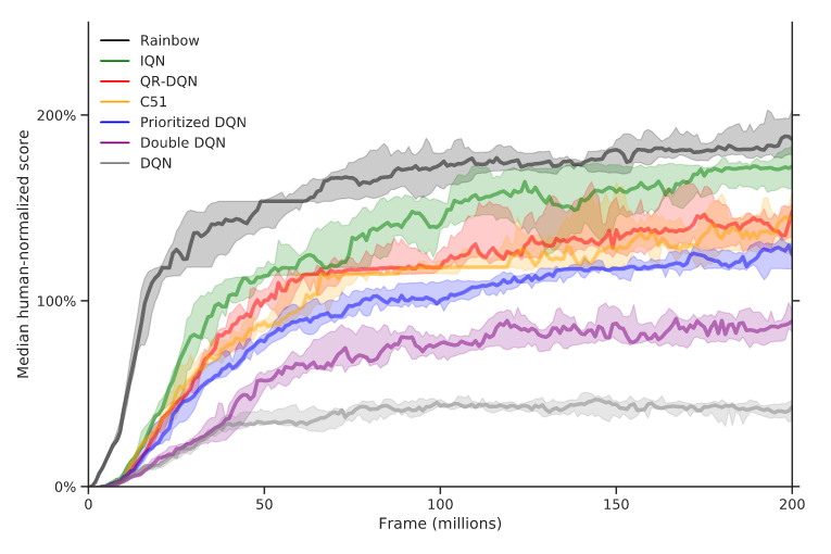
Deep Q-Networks, first reported by Mnih et al. in 2013 in the paper [1], is one of the best-known Reinforcement Learning algorithms to date, due to the ability it has shown since its publication to achieve higher-than-human performance in countless Atari games, as shown in Figure 1.
Also, aside from how fascinating it is to see a DQN agent playing any of these Atari games as if it was a professional gamer, DQN solves some of the problems of an algorithm that has been known for decades: Q-Learning, which was already introduced and explained in the first article of this series:
Q-Learning intends to find a function (Q-Function) in a form of a state-action table that calculates the expected total sum of rewards for a given state-action pair, such that the agent is capable of making optimal decisions by executing the action that implies the highest output of the Q-Function. Although Watkins and Dayan demonstrated mathematically in 1992 that this algorithm converges to optimal Action-Values as long as the action space is discrete and each and every possible state and action are explored repeatedly [2], this convergence is difficult to achieve in realistic environments. After all, in an environment with a continuous state space it is impossible to go through all the possible states and actions repeatedly, since there are an infinite number of them and the Q-Table would be too big.
DQN solves this problem by approximating the Q-Function through a Neural Network and learning from previous training experiences, so that the agent can learn more times from experiences already lived without the need to live them again, as well as avoiding the excessive computational cost of calculating and updating the Q-Table for continuous state spaces.
DQN Components
Leaving aside the environment with which the agent interacts, the three main components of the DQN algorithm are the Main Neural Network, the Target Neural Network, and the Replay Buffer.
Main Neural Network
The Main NN tries to predict the expected return of taking each action for the given state. Therefore, the network’s output will have as many values as possible actions to take, and the network’s input will be a state.
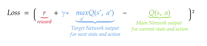
The neural network is trained by performing Gradient Descent to minimize the Loss Function, but for this a predicted value and a target value are needed with which to calculate the loss. The predicted value is the output of the main neural network for the current state and action, and the target value is calculated as the sum of the reward obtained plus the highest value of the target neural network’s output for the next state multiplied by a discount rate γ. The calculation of the loss can be mathematically understood by means of Figure 2.
As for why these two values are used for the loss calculation, the reason is that the target network, by getting the prediction of future rewards for a future state and action, has more information about how useful the current action is in the current state.
Target Neural Network
The Target Neural Network is used, as mentioned above, to get the target value for calculating the loss and optimizing it. This neural network, unlike the main one, will be updated every N timesteps with the weights of the main network.
Replay Buffer
The Replay Buffer is a list that is filled with the experiences lived by the agent. Making a parallelism with a Supervised Learning training, this buffer will be the equivalent of the dataset that is used to train, with the difference that the buffer must be filled little by little, as the agent interacts with the environment and collects information.
In the case of the DQN algorithm, each of the experiences (rows in the dataset) that make up this buffer are represented by the current state, the action taken in the current state, the reward obtained after taking that action, whether it is a terminal state or not, and the next state reached after taking the action.
This method to learn from experiences, unlike the one used in the Q-Learning algorithm, allows learning from all the agent’s interactions with the environment independently of the interactions that the agent has just had with the environment.
DQN Algorithm Flow
The flow for the DQN algorithm is presented following the pseudocode from [1], which is shown below.
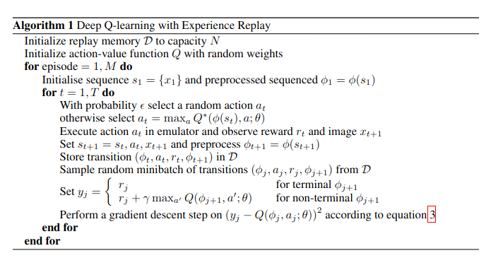
For each episode, the agent performs the following steps:
1. From given state, select an action
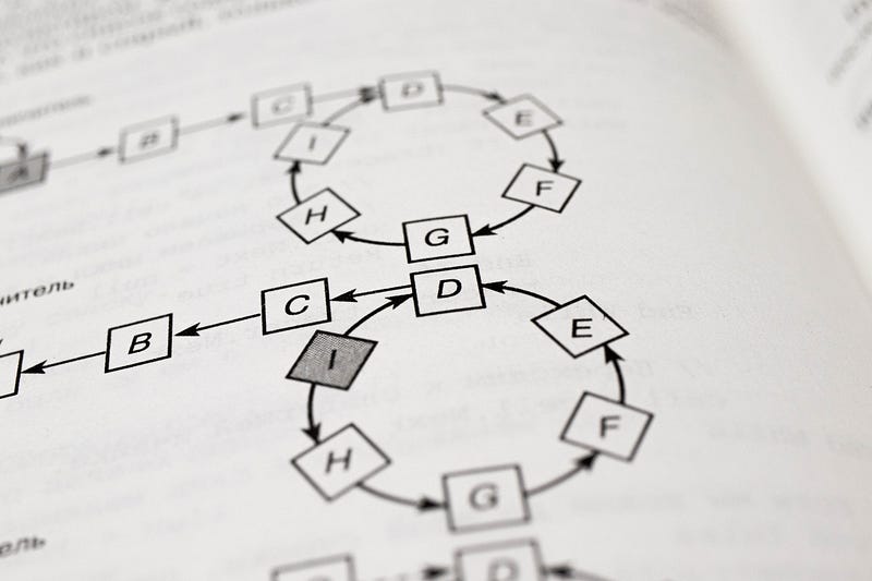
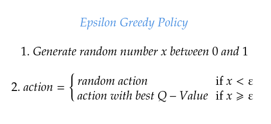
The action is chosen following the epsilon-greedy policy, which was previously explained in [3]. This policy will take the action with the best Q-Value, which is the output of the main neural network, with probability 1-ε, and will pick a random action with probability ε (see Figure 3). Epsilon (ε) is one of the hyperparameters to be set for the algorithm.
2. Perform action on environment
The agent performs the action on the environment, and gets the new state reached, the reward obtained, and whether a terminal state has been reached. These values are usually returned by most gym environments [4] when performing an action via the step() method.
3. Store experience in Replay Buffer
As previously mentioned, experiences are saved in the Replay Buffer as {s, a, r, terminal, s’}, being s and a the current state and action, r and s’ the reward and new state reached after performing the action, and terminal a boolean indicating whether a goal state has been reached.
4. Sample a random batch of experiences from Replay Buffer
If the Replay Buffer has enough experiences to fill a batch (if the batch size is 32 and the replay buffer only has 5 experiences, the batch cannot be filled and this step is skipped), a batch of random experiences is taken as training data.
5. Set the target value
The target value is defined in two different ways, depending on whether a terminal state has been reached. If a terminal state has been reached, the target value will be the reward received, while if the new state is not terminal, the target value will be, as explained before, the sum of the reward and the output of the target neural network with the highest Q-Value for the next state multiplied by a discount factor γ.

The discount factor γ is another hyperparameter to be set for the algorithm.
6. Perform Gradient Descent
Gradient Descent is applied to the loss calculated from the output of the main neural network and the previously calculated target value, following the equation shown in Figure 2. As can be seen, the loss function used is the MSE, so the loss will be the difference between the output of the main network and the target squared.
7. Execute the following timestep
Once the previous steps have been completed, this same process is repeated over and over again until the maximum number of timesteps per episode is reached or until the agent reaches a terminal state. When this happens, it goes to the next episode.
Conclusion
The DQN algorithm represents a considerable improvement over Q-Learning when it comes to training an agent in environments with continuous states, thus allowing greater versatility of use. In addition, the fact of using a neural network (specifically a convolutional one) instead of Q-Learning’s Q-Table allows images to be fed to the agent (for example frames of an Atari game), which adds even more versatility and usability to DQN.
Regarding the weaknesses of the algorithm, it should be noted that the use of neural networks can lead to higher execution times in each frame compared to Q-Learning, especially when large batch sizes are used, since carrying out the process of forward propagation and backpropagation with lots of data is considerably slower than updating the Q-Values of the Q-Table using the modified Bellman Optimality Equation introduced in Applied Reinforcement Learning I: Q-Learning. In addition, the use of the Replay Buffer can be a problem, as the algorithm works with a huge amount of data that is stored in memory, which can easily exceed the RAM of some computers.
REFERENCES
[1] MNIH, Volodymyr, et al. Playing atari with deep reinforcement learning. arXiv preprint arXiv:1312.5602, 2013.
[2] WATKINS, Christopher JCH; DAYAN, Peter. Q-learning. Machine learning, 1992, vol. 8, no 3, p. 279–292.
[3] Applied Reinforcement Learning I: Q-Learning https://readmedium.com/applied-reinforcement-learning-i-q-learning-d6086c1f437
[4] Gym Documentation https://www.gymlibrary.dev/


