Apache Cassandra for Structured and Semi-Structured Data

Apache Cassandra — Distributed Row-Partitioned Database for Structured and Semi-Structured Data

Apache Cassandra is an open-source distributed row-partitioned database management system (distributed DBMS) to handle large amounts of structured data across many commodity servers, providing high scalability (linearly scalable) and high availability (fault-tolerant) with no single point of failure. It supports for only structured or semi-structured data and the database consistency levels can be tuned to considerably high degrees.

Listed below are some of the notable points of Apache Cassandra:

• Scalability: It is linearly scalable, i.e., it increases the throughput as you increase the number of nodes in the cluster.
• Fault Tolerance: It implements a Dynamo-style replication model with no single point of failure, but adds a more powerful “column family” data model.
• Consistency: It can be tuned to varying degrees of consistency (based on requirement).
• It is designed to run on cheap commodity hardware. It performs blazingly fast writes and can store hundreds of terabytes of data, without sacrificing the read efficiency.
• Facebook, Amazon and Google: Created at Facebook, it differs sharply from RDBMs. Its distribution design is based on Amazon’s Dynamo and its data model on Google’s Bigtable.
• It is row-partitioned database.

In Apache Cassandra, you want to model your data to your queries, and if your business need calls for quickly changing requirements, you need to create a new table to process the data.

Handy References:

• Cassandra Home
• Cassandra Documentation
• Cassandra Architecture
• Cassandra Query Language (CQL) Documentation
• Official Cassandra Image
• Cassandra Client Drivers (such as cassandra-driver for Python by DataStax)

For cloud solution for Cassandra, refer Amazon Keyspaces or DataStax’s Cassandra as a Service, called Astra on Google Cloud Marketplace.

Cassandra Terms

Keyspaces:

Keyspaces are containers of data, similar to the schema or database in a RDBMS. Typically, a keyspace contain many tables. A table belongs to only one keyspace.

Replication is specified at the keyspace level.

Tables:

Tables are also referred to as column families in the earlier version of Cassandra. Tables contain a set of columns and a primary key, and they store data in a set of rows.

Every table must have a primary key.

Columns:

Column represents a single piece of data in Cassandra and has a type defined.

There are some special columns:

• Universal Unique Identity (UUID): This is similar to sequence numbers in relational databases. It is a 128-bit integer.
• TimeUUID: It contains a timestamp and guarantees no duplication. TimeUUID uses time in 100 nanosecond intervals. You can use the function now() to get the TimeUUID.
• Counter: It stores a number which can only be updated by adding or subtracting from the current value, with its initial value zero.

Primary Key, Partitioning Key, Clustering Columns, and Data Columns:

Every table must have a primary key with unique constraint.

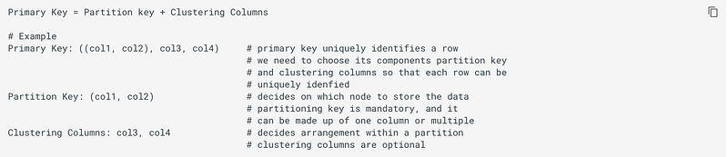
Partition key is the first component of Primary key. Its hashed value is used to determine the node to store the data. The partition key can be a compound key consisting of multiple columns. We want almost equal spreads of data, and we keep this in mind while choosing primary key.

Any fields listed after the Partition Key in Primary Key are called Clustering Columns. These store data in ascending order within the partition. The clustering column component also helps in making sure the primary key of each row is unique.

You can use as many clustering columns as you would like. You cannot use the clustering columns out of order in the SELECT statement. You may choose to omit using a clustering column in you SELECT statement. That’s OK. Just remember to sue them in order when you are using the SELECT statement. But note that, in your CQL query, you can not try to access a column or a clustering column if you have not used the other defined clustering columns. For example, if primary key is (year, artist_name, album_name) and you want to use city column in your query’s WHERE clause, then you can use it only if your WHERE clause makes use of all of the columns which are part of primary key.

When inserting records, Cassandra hashes the value of the inserted data’s partition key; Cassandra uses this hash value to determine which node is responsible for storing the data.

Tokens:

Cassandra uses tokens to determine which node holds what data. A token is a 64-bit integer, and Cassandra assigns ranges of these tokens to nodes so that each possible token is owned by a node. Adding more nodes to the cluster or removing old ones leads to redistributing these token among nodes.

A row’s partition key is used to calculate a token using a given partitioner (a hash function for computing the token of a partition key) to determine which node owns that row.

Cassandra is Row-partition store:

Row is the smallest unit that stores related data in Cassandra.

Don’t think of Cassandra’s column family (that is, table) as a RDBMS table, but think of it as a dict of a dict (here dict is data structure similar to Python’s OrderedDict):

• the outer dict is keyed by a row key (primary key): this determines which partition and which row in the partition
• the inner dict is keyed by a column key (data columns): this is data in dict with column names as keys
• both dict are ordered (by key) and are sorted: the outer dict is sorted by primary key

This model allows you to omit columns or add arbitrary columns at any time, as it allows you to have different data columns for different rows.

Getting started with Cassandra

Starting a Cassandra cluster is as simple as:

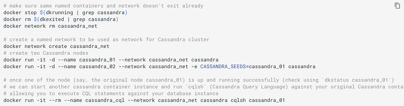
To start a new container, we just tell each new node where the first is.

For separate machines, you need to tell Cassandra what IP address to advertise to the other nodes (since the address of the container is behind the docker bridge).

Cassandra Architecture

Refer Official docs on Cassandra Architecture.

Cassandra organizes data into partitions. Each partition is stored on node and consists of multiple columns. Nodes are generally part of a cluster where each node is responsible for a fraction of the partitions.

Cassandra has masterless and peer-to-peer (that is, each node is connected to every other node) distributed system across its nodes, and data is distributed among all the nodes in a cluster:

• All the nodes in a cluster play the same role. Each role is independent and at the same time interconnected to other nodes.
• Each node in a cluster can accept read and write requests, regardless of where the data is actually located in the cluster.
• When a node goes down, read/write requests can be served from other nodes in the network.

Cassandra has peer-to-peer distributed system across homogeneous nodes where data is distributed among all nodes in the cluster. Each node frequently exchanges state information about itself and other nodes across the cluster using peer-to-peer gossip communication protocol. A sequential written commit log on each node captures write activity to ensure data durability. Data is then indexed and written to an in-memory structure, called a memtable, which resembles a write-back cache. Each time the memory structure is full, the data is written to disk in an SSTable (sorted string table) data file. All writes are automatically partitioned and replicated throughout the cluster.

All nodes in a Cassandra cluster can accept reads and writes, no matter where the data being written or requested actually belongs in the cluster. All nodes are essentially identical and as a result Cassandra has no single point of failure, and therefore no need for complex sharding or leader election. Cassandra is able to achieve both availability and scalability using a data structure that allows any node in the system to easily determine the location of a particular key in the cluster. This is accomplished by using a distributed hash table (DHT) design based on the Amazon Dynamo architecture.

Replication:

The replication strategy of a keyspace determines which nodes are replicas for a given token range.

SimpleStrategy allows a single integer replication_factor to be defined. This determines the number of nodes that should contain a copy of each row. SimpleStrategy treats all nodes identically, ignoring any configured datacenters and racks.

NetworkTopologyStrategy allows a replication factor to be specified for each datacenter in the cluster. Even if your cluster only uses a single datacenter, NetworkTopologyStrategy should be preferred over SimpleStrategy to make it easier to add new physical or virtual datacenters to the cluster later.

Tunable Consistency:

Write operations are always sent to all replicas, regardless of consistency level. The consistency level simply controls how many responses (ONE, TWO, THREE, QUORUM, ALL, LOCAL_QUORUM, EACH_QUORUM, LOCAL_ONE, ANY) the coordinator waits for before responding to the client. Here, QUORUM means “majority”.

It is common to pick read and write consistency levels that are high enough to overlap, resulting in “strong” consistency. This is typically expressed as W + R > RF, where W is the write consistency level, R is the read consistency level, and RF is the replication factor. For example, if RF = 3, a QUORUM request will require responses from at least two of the three replicas. If QUORUM is used for both writes and reads, at least one of the replicas is guaranteed to participate in both the write and the read request, which in turn guarantees that the latest write will be read. In a multi-datacenter environment, LOCAL_QUORUM can be used to provide a weaker but still useful guarantee: reads are guaranteed to see the latest write from within the same datacenter.

If this type of strong consistency isn’t required, lower consistency levels like ONE may be used to improve throughput, latency, and availability.

CommitLog:

CommitsLogs are an append-only log for all mutations local to Cassandra node. Any data written to Cassandra will first be written to commit log before being written to a memtable. This provides durability in the case of the expected shutdown. On startup, any mutations in the commit log will be applied to memtables.

Memtables:

Memtables are in-memory structures where Cassandra buffer writes. Eventually, memtables are flushed onto disk and become immutable SSTables.

SSTables:

SSTables are the immutable data files that Cassandra uses. for persisting data on disk.

Data Modeling in Apache Cassandra

Data modeling is a process that involves identifying the entities (items to be stored) and the relationships between entities.

Denormalization of tables (based on the queries) in Cassandra is absolutely critical. The biggest take away when doing data modeling in Apache Cassandra is to think about your queries first (in fact, for all NoSQL databases). In fact, we create one table for each similar set of queries (these similar sets of queries can answered through same definition of the partition key and clustering columns, that is via same data model).

There are no JOINs in Apache Cassandra. So, we need different queries for different tables.

Also, there is no support for GROUP BY and sub-queries in CQL.

Since Apache Cassandra requires data modeling based on the query you want, you can’t do ad-hoc queries. So, you can’t do analysis, such as GROUP BY statements on Apache Cassandra. However, you can add clustering columns into your data model and create new tables.

Data modeling in Apache Cassandra is query focused, and that focus needs to be on the WHERE clause. The PARTITION KEY must be included in your query and any CLUSTERING COLUMNS can be used in the order (omitting one of some clustering columns is OK, though) they appear in your PRIMARY KEY. But note that, in your CQL query, you can not try to access a column or a clustering column if you have not used the other defined clustering columns.

The WHERE the clause must be included to execute queries. It is recommended that one partition be queried at a time for performance implications. It is possible to do a SELECT * from <table> if you add configuration ALLOW FILTERING to your query. This is risky, but available if absolutely necessary.

Indexes (Secondary) in Cassandra

An index (formally named “secondary index”) provides means to access data in Cassandra using non-primary key fields. If there is no index on such a columns, it is not even allowed to be conditionally queried (that is, such columns are not normally queryable).

An index indexes columns value in a separate, hidden column family (table) from the one that contains the values being indexed. The data of an index is local only (that is, within a node; of course, because the column used for index in a non-clustering key). This also means that for data query by indexed column, the requests have to be forwarded to all the nodes, waiting for all the responses, and then the results are merged and returned. So if you have many nodes, the query response slows down as more machines are added to the cluster.

Internal of Writes and Reads in Cassandra

Every node first writes the mutation to the commit log and then writes the mutation to the memtable. Writing to the commit log ensures the durability of the writer as the memtable is an in-memory structure and is only written to disk when the memtable is flushed to disk. A memtable is flushed to disk when:

• it reaches its maximum allocated size in memory
• the number of minutes a memtable can stay in memory elapses
• manually flushed by a user

How Writes and Reads Happen?

Since Cassandra is a masterless, a client can connect with any node in a cluster. The chosen node is called “coordinator” and it is responsible for satisfying the client requests. The consistency level determines the number of nodes that the coordinator needs to hear from in order to notify the client of a successful mutation. All inter-node requests are sent through a messaging service and in an asynchronous manner. Based on the partition key and replication strategy used, the coordinator forwards the mutation to all applicable nodes.

At the cluster level a read operation and write operation are similar.

QUORUM, n/2 + 1 where n is a replication factor, is a commonly used consistency level which refers to a majority of nodes.

A memtable is flushed to an immutable structure called SSTable (Sorted String Table). The commit log is used for playback purposes in case data from the memtable is lost due to node failure. Every SSTable creates three files on disk which includes a bloom filter, a key index, and a data file. Over a period of time, a number of SSTables are created. This results in the need to read multiple SSTables and scan the memtable for applicable data fragments to satisfy a read request.

A row key must be supplied for every read operation. The coordinator uses the row key to determine the first replica. As with the write path, the consistency level determines the number of replica’s that must respond before successfully returning data. If the contacted replicas have a different version of data the coordinator returns the latest version to the client and issues a read repair command to the node/nodes with the older version of the data.

Every SSTable has an associated bloom filter which enables it to quickly ascertain if data for the requested row key exists on the corresponding SSTable. This reduces IO when performing a row key lookup. A bloom filter is always held in memory since the whole purpose is to save disk IO. Cassandra also keeps a copy of the bloom filter on disk which enables it to recreate the bloom filter in memory quickly.

If the bloom filter returns a negative response, no data is returned from that particular SSTable. This is a common cause as the compaction operation tries to group all row key-related data into a few SSTable as possible.

If the bloom filter provides a positive response the partition key cache is scanned to ascertain the compression offset for the requested row key. It then proceeds to fetch the compressed data on disk and returns the result set. The partition summary is a subset to the partition index and helps determine the approximate location of the index entry in the partition index. The partition key is then scanned to locate the compression offset which is then used find the appropriate data on disk.

Inserting and Querying Cassandra

The API to Cassandra is CQL, the Cassandra Query Language. To use CQL, you will need to connect to the cluster, which can be done:

• either using cqlsh,
• or through a client driver for Cassandra

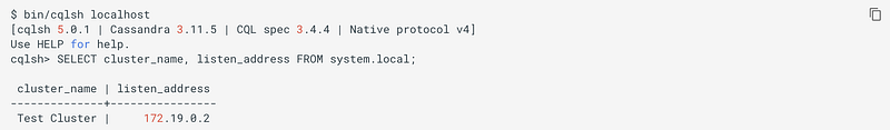
The cqlsh is a command-line shell for interacting with Cassandra through CQL. It is shipped with every Cassandra package and can be found in bin/ the directory alongside the Cassandra executable. It connects to the single node specified on the command line. For example,

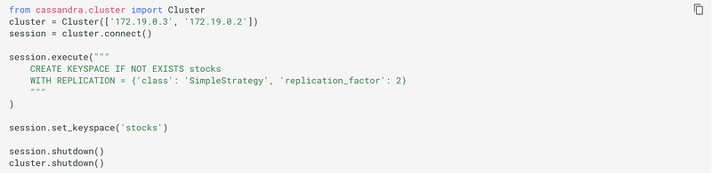
The datastax/python-driver is Github repo for Python client library for Cassandra, which can be installed as simple as pip install cassandra-driver.

For example,

Cassandra Query Language (CQL)

The API to Cassandra is CQL, the Cassandra Query Language, which is a dialect similar to SQL. While similar to SQL, there is a notable omission: Apache Cassandra does not support JOIN operations or subqueries or GROUP BY clause, rows are identified by primary key and no duplicates are allowed, INSERT does not check the prior existence of the row by default so a row is created if none existed before and updated otherwise.

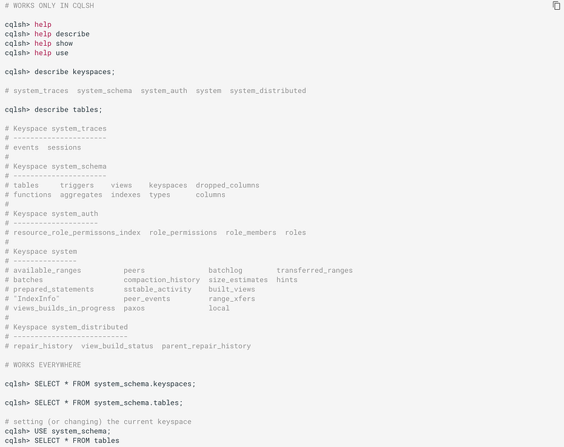
Here’s how you can get info about existing keyspaces and tables:

Apart from native data types, Cassandra supports:

• 3 kinds of collections: Maps, Sets, and Lists. Collections are meant for storing/denormalizing a relatively small amount of data. They work well for things like “the phone numbers of a given user”, “labels applied to an email”, etc. But when items are expected to grow unbounded (“all messages sent by a user”, “events registered by a sensor”, …), then collections are not appropriate and a specific table (with clustering columns) should be used.
• definition of user-defined types (UDT).
• tuple types (where the elements can be of different types). Functionally, tuples can be thought of as anonymous UDT with anonymous fields.

Cassandra 2.2 introduced JSON support for SELECT and INSERT statements. This support does not fundamentally alter the CQL API (for example, the schema is still enforced), it simply provides a convenient way to work with JSON documents.

A table can be created using create table command. Creating a table amounts to defining which columns the rows will be composed and optional options for the table. Every row in a CQL table has a set of predefined columns defined at the time of the table creation (or added later using alter statement).

A column definition is primarily comprised of the name of the column defined and it’s a data type. Additionally, a column definition can have the following modifiers:

• STATIC: a column that is static will be “shared” by all the rows belonging to the same partition (having the same partition key). Only non PRIMARY KEY columns can be static.
• PRIMARY KEY: it declares the column as being the sole component of the primary key of the table

Within a table, a row is uniquely identified by its PRIMARY KEY, and hence all table must define a PRIMARY KEY (and only one). A PRIMARY KEY definition is composed of one or more of the columns defined in the table.

Syntactically, the primary key is defined the keywords PRIMARY KEY followed by a comma-separated list of the column names composing it within parenthesis, but if the primary key has only one column, one can alternatively follow that column definition by the PRIMARY KEY keywords. The order of the columns in the primary key definition matter.

A CQL primary key is composed of 2 parts:

• the partition key part. It is the first component of the primary key definition. It can be single-column or, using additional parenthesis, can be multiple columns.
• the clustering columns. These are the columns after the first component of the primary key definition, and the order of those columns define the clustering order.

A table always has at least a partition key, and if the table has no clustering columns, then every partition of that table in only comprised of a single row (since the primary key uniquely identifies rows and the primary key is equal to the partition key if there are no clustering columns).

For example,

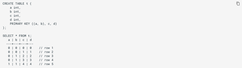
Here, row 1 and row 2 are in the same partition, row 3 and row 4 are also in the same partition (but a different one) and row 5 is in yet another partition.

The most important property of partition is that all the rows belonging to the same partition are guaranteed to be stored on the same set of replica nodes. In other words, the partition key of a table defines which of the rows will be localized together in the Cluster, and it is thus important to choose your partition key wisely so that rows that need to fetch together are in the same partition (so that querying those rows together require contacting a minimum of nodes). A partition key that groups too much data can create a hotspot (as all of that data has to be stored on the same set of replica nodes).

The clustering columns of a table define the clustering order for the partition of that table. For a given partition, all the rows are physically ordered inside Cassandra by that clustering order.

A CQL table has a number of options that can be set at creation (and, for most of them, altered later). These options are specified after the with keyword.

The clustering order of a table is defined by the clustering columns of that table. By default, that ordering is based on the natural order of those clustering order, but the CLUSTERING ORDER allows us to change that clustering order to use the reverse natural order for some (potentially all) of the columns.

CQL supports creating secondary indexes on tables, allowing queries on the table to use those indexes.

In a CQL table, new rows can be inserted, and existing rows can be updated or deleted.

Materialized views can be created for a CQL table. Each such view is a set of rows that corresponds to rows that are present in the underlying, or base, table specified in the SELECT statement. A materialized view cannot be directly updated, but updates to the base table will cause corresponding updates in the view.

Here are some related interesting stories that you might find helpful:

• Distributed Data Processing with Apache Spark
• Data Streaming With Apache Kafka
• Data Pipelines with Apache Airflow
• Designing Workflows using Argo
• The Why and How of MapReduce
• Observer Pattern vs. Pub-Sub Pattern