Adaptive Control (Part II) —Modeling the X-15’s Adaptive Flight Control System

How to build from scratch a Simulink model of the famous MH-96, the X-15's Adaptive Flight Control System

Welcome to the second chapter of this series about Adaptive Control.

In the previous article, we made a one-way trip to the past, more specifically to the early 60s, the era of the firsts adaptive flight control system, and the beginning of hypersonic manned flights with the North American X-15.

In this new issue, we will make the way back trip to the present.

Using nowadays technology, we will build up a simplified simulation model of the X-15’s Adaptive Flight Control System (AFCS), the MH-96.

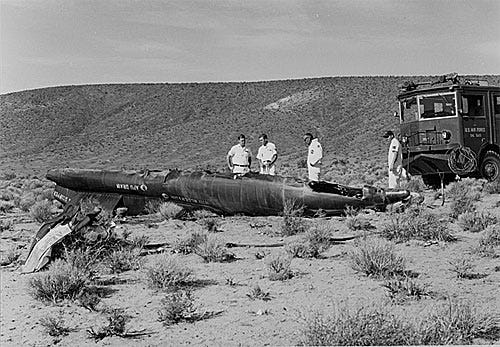
It’s curious to think that you could even simulate the X-15’s flight dynamics in your mobile phone. Do you know what did it take to do this in the 60s?

Take a look at this photo…

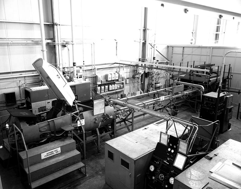
This is a good example to show us how fast technology evolves. So we will take advantage of the 2020s’ computational capabilities to build up a simplified Simulink model of the X-15’s pitch dynamics and the MH-96 AFCS.

With this model, we’ll have a firsthand view of the MH-96’s performance in a real-life example.

Ready? Let’s get down to business!

The X-15’s MH-96 Adaptive Flight Control System

The MH-96 was one of Honeywell’s first-generation adaptive autopilots and was based on a Model Reference Adaptive Control architecture with a single adaptive gain.

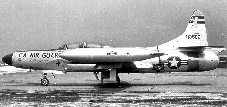
The MH-96 AFCS was indeed an upgraded version of the F-94C’s E-10 autopilot, which was the first adaptive flight control system to fly in a manned aircraft back in 1958.

As all Honeywell’s first-generation model-following adaptive autopilots, the MH-96 was a rate-command Self-Oscillating Adaptive Controller with a single adaptive gain.

The architecture of the MH-96’s pitch rate control loop was conceptually simple, deceptively so.

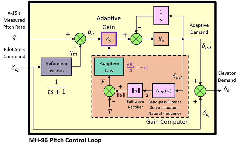
The MH-96’s main goal was to operate always with its feedback loop’s gain (Kq) as high as possible, right on the verge of instability, where the controller achieves the best tracking of the Reference System.

The Reference System (purple block in Figure 4), which defines the target response of the X-15’s pitch rate, was defined by a first-order low-pass filter, with a time constant τ of 0.5sec (0.33sec for the lateral-directional inner control loop).

The (simplified) adaptation law of the feedback gain Kq was computed via the MIT rule.

Where T is a threshold between acceptable and unacceptable oscillation’s amplitude, Kq is the MH-96’s pitch-axis adaptive gain, and ||u(Kq)||is the amplitude of the adaptive demand component around a frequency bandwidth centered at the natural frequency of the servo-actuator loop.

Building the MH-96’s Simulink Model

At this point, although we have all the “ingredients” to cook a simplified model of the MH-96 AFCS, we still need to gather the actuator’s technical data and the X-15’s elevator-to-pitch-rate transfer function to build up a closed-loop model.

At first, this seemed to me like a nearly impossible task, but in a fortunate stroke of serendipity, I found two insightful technical reports where the transfer function of the actuators and the X-15’s pitch dynamics were clearly stated for a flight condition at Mach 1.2 and 40,000ft (you can have a read here and here respectively).

From the first reference, the elevator-to-pitch-rate transfer function can be modeled as a second-order transfer function:

The X-15’s elevator actuator had a maximum deflection limit of 15deg on top of the trim position, with a transfer function which could be approximated as:

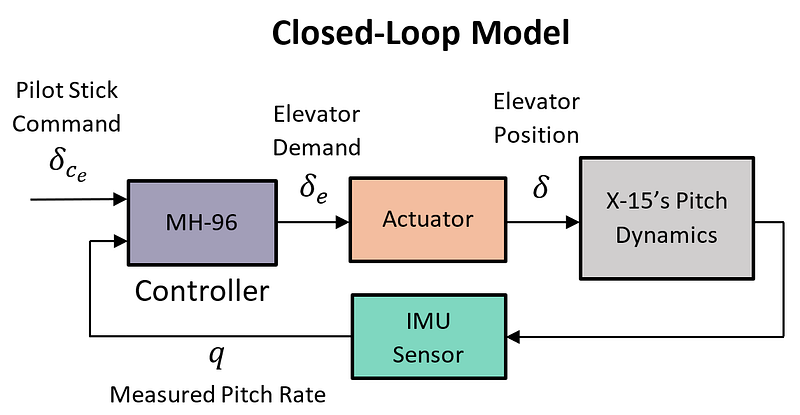
Once we have collected all the required data to build the closed-loop model, we are ready to create a Simulink model which will be composed by:

• The flight control system: the MH-96 AFCS
• The elevator actuator model, including an amplitude saturation block
• The X-15’s pitch rate dynamics
• Sensors: we will assume perfect IMU sensors (unitary transfer function)

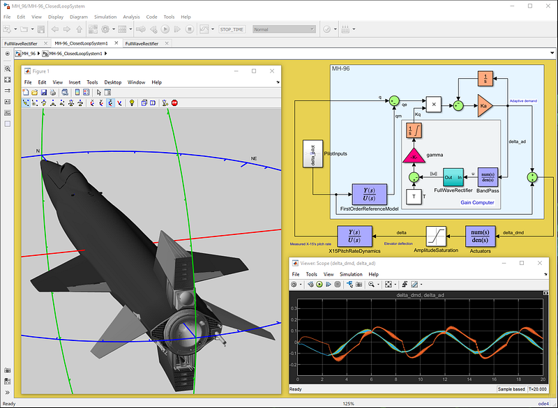
Here you can see the final Simulink model.

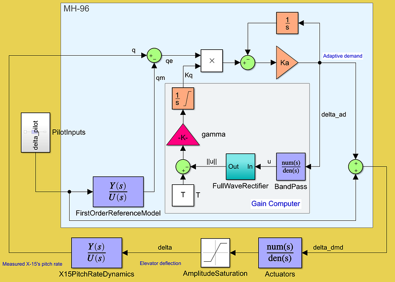
With the previous model, we will be able to inspect the evolution of the adaptive gain Kq in a real-life example, and we’ll see how its value will increase if the amplitude of the oscillations ||u(Kq)|| is lower than the amplitude threshold T (when Kq is lower than the K-Instability limit), and vice versa.

At this limit condition, when the adaptive gain Kq reaches the K-Instability limit, the closed-loop system changes its stability nature, from stable to unstable, and the resulting unstable mode is an oscillatory mode with a frequency that is really close to the actuator’s natural frequency.

It’s worth remarking that the K-Instability limit is a priori UNKNOWN to the controller. This is, the controller can only “feel” that the current Kq value is close to the K-Instability limit when the oscillations’ amplitude (||u(Kq)||) is close to the threshold T.

Analyzing the Stability Limit of the MH-96’s Adaptive Gain

At this point, you might be wondering, is there any method to determine which is the actual value of the K-Instability limit? Yes, there’s one, and really simple indeed (thanks to Mr. Harry Nyquist for that!).

We can compute the K-Instability limit by linearizing the following open-loop model.

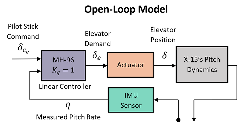
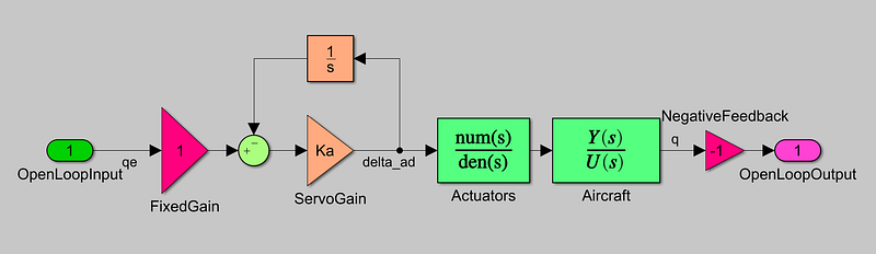
The Open-Loop transfer function of the previous Simulink model can be linearized to determine the value of the Kq gain that would make the closed-loop system to be neutrally stable (using the Nyquist stability criterion).

Hereafter I’ve included a snippet of the MATLAB code required to load the model’s data and to linearize the MH-96’s open-loop model:

After running this code, we will obtain the following Nichols chart for Kq=1.

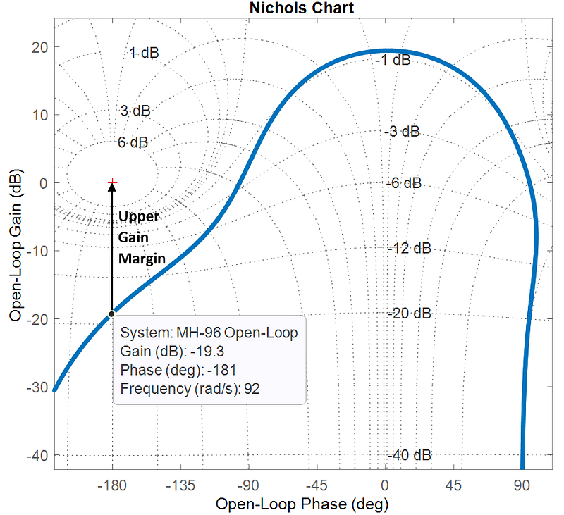
Using the system’s Upper Gain Margin (UGM), defined by the amplification at phase -180deg, we can compute the Kq gain value that would make the closed-loop system to be neutrally stable as:

Then, if we run a simulation with the closed-loop model (the one shown in Figure 6), we will see firsthand how the MIT rule is able to drive the Kq gain close to its optimal value of 9.2257.

But first things first…

The X-15’s Natural Stability

As we have previously introduced, at Mach 1.2 and 40,000ft, the Kq gain stabilizes the vehicle for values ranging from 0 to 9.2257.

The lower bound 0 corresponds to a condition where the MH-96 does not provide any stability augmentation at all, and thus the X-15’s pitch dynamics will be those of the un-augmented system (natural stability).

Then, we could see the natural stability of the vehicle in this flight condition (with fixed controls), and how the system’s response compares to those of the reference system if we just set Kq = 0.

Let’s code some MATLAB lines to run the simulation:

This is what we get for a doublet stick input, defined by first a first pitch-up step input, followed by a pitch down to center pitch stick, and so on.

As you can see, the handling qualities of the un-augmented vehicle are far from being “optimal”, with a step response with very low damping and even reaching negative pitch rate values after the first overshoot, which is not desired at all. And what’s more, the un-augmented dynamics are very different from those of the reference system (the shadowed 3D model in Figure 11).

With these results, it’s evident that the X-15 needed a stability augmentation system to improve the vehicle’s handling qualities, and the MH-96 did a great job, as you will see next.

Evaluating the MH-96 Adaptive Controller’s Performances

Now let’s start squeezing our closed-loop simulator to get some “real juice”. We have been playing around with the dynamics of the un-augmented system, and we’ve checked firsthand they are not good at all. Now it's the turn for the adaptive controller to show up.

How would the MH-96 perform with a starting condition of Kq = 0? Will it provide a good tracking of the reference system? So let’s turn on the adaptive gain γ and run again the simulation to get the answer.

And this is what we finally get: the MH-96 AFCS “in action”.

This is the real “magic” of the MH-96 adaptive flight control system.

As the simulation results show, although the Kq-Instability threshold is a prior unknown to the controller, it’s able to provide a good tracking of the reference system, just on the verge of instability, where the optimum reference system tracking performance is achieved.

I’m sure you might be wondering if it always is this way, right? So do I.

So let’s try to fool the MH-96 controller.

In our attempt, we will change the X-15’s elevator control power Mδ decreasing it a 62%, simulating now a new operating condition at an altitude of 60,000ft (+20,000ft from the previous flight condition).

What would happen then? These are the results:

As the mathematic formulation predicted, although it requires a longer time, the MIT law provides once again a good tracking of the reference system after driving the Kq gain close to its a priori unknown stability limit.

This is one was one of the main advantages of the MH-96 controller indeed: to provide almost a homogenous pitch and roll rate response to the pilot commands at almost every operating condition, even during the most critical one, the re-entry phase.

What’s Next?

All that glitters is not gold, and the MIT rule is no exception.

This apparently simple and efficient adaptation law has a dark side: it does not always ensure the convergence of the controlled vehicle’s dynamics towards that of the reference system.

But engineers at that time (during the 60s and 70s) were not aware of any of the mechanisms that can destabilize the MIT rule. But why?

The point is that the MIT rule came at a time when the mathematical theory required to formally demonstrate the local/global stability of adaptive control systems using such adaptation law had not yet been developed.

It wasn’t until the late 70s that a mathematical theory (Lyapunov theory) was available to determine the specific conditions that triggered the MIT rule’s instabilities.

In the next chapter of this series, we will put some light on the dark side of the MIT rule, revealing the lessons learned during the development of the MH-96 AFCS and after the only fatal accident of the X-15 circa 1967 (flight 3–65–97).

The Github Repository

I have collected all the previous code and examples in this Github repository. Check it out if you want to play around with the MH-96 adaptive flight control system.

In addition, if you want to reproduce the 3D visualizations I’ve shown you in this article, or if you want to use your own 3D models, this is a must-read:

And here is the corresponding GitHub repository, have fun buddy!

References

[1] Iven M.Y. Mareels, Brian D.O. Anderson, Robert R. Bitmead, Marc Bodson, Shankar S. Sastry, Revisiting the Mit Rule for Adaptive Control, IFAC Proceedings Volumes, Volume 20, Issue 2, 1987, Pages 161–166, ISSN 1474–6670

[2] Orr J.S., Statler I.C., Barshi I. (2015) The X-15 3–65 Accident: An Aircraft Systems and Flight Control Perspective. In: Sgobba T., Rongier I. (eds) Space Safety is No Accident. Springer, Cham.

[3] Dydek, Zachary, Anuradha Annaswamy, and Eugene Lavretsky. “Adaptive Control and the NASA X-15–3 Flight Revisited.” IEEE Control Systems Magazine 30.3 (2010): 32–48. Web.© 2010 IEEE.

[4] NASA Technical Report. Experience With the X-15 Adaptive Flight Control System.

Rodney Rodríguez Robles is an aerospace engineer, cyclist, blogger, and cutting edge technology advocate, living a dream in the aerospace industry he only dreamed of as a kid. He talks about coding, the history of aeronautics, control engineering, rocket science, and all the technology that is making your day by day easier.

Please check me out on the following social networks as well, I would love to hear from you! — LinkedIn, Twitter.