
3D Animations Made Simple With MATLAB— Visualizing Flight Test Data and Simulation Results
How to build the definite animation tool that will help you analyze in detail the complex dynamics of an aircraft’s movement
They say data is gold.
However, raw-data on its own will never be as valuable as gold. It’s the post-processing and visualization tools that allow us to exploit all the added value that the data hides.
In the aerospace industry, we analyze a vast amount of raw data generated by high-fidelity simulators. When it comes to the validation and verification of flight control systems, the number of simulations required to be performed to check the aircraft’s controllability and handling qualities starts to build-up.
In some cases, we simulate millions of maneuvers to check that the aircraft never departs from a controlled flight condition under any circumstances.
If you want to go into more depth on this topic you can take a look at this article.
Once a “departure from controlled flight” is spotted using automatic post-processing algorithms, the maneuver is analyzed thoroughly to determine the root cause of the issue.
The following figure depicts an example of what a “departure from controlled flight” looks like on a highly maneuverable fighter jet.
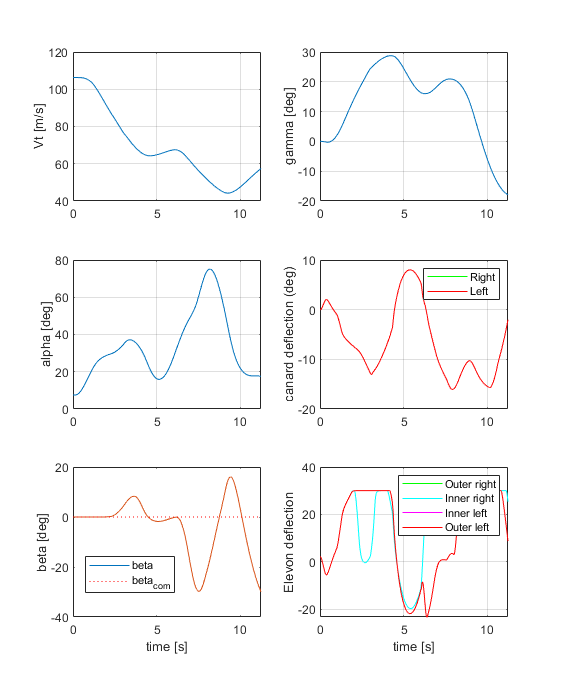
Can you spot it?
Of course, to the bare and untrained eye, it’s complicated to see anything in these time-history plots. And for the skilled eye, even sometimes, it’s also a complicated task.
Here is when a good 3D animation tool comes into hand.
Do you see now a “departure from controlled flight”? Scary, isn’t it?
In this post, you will learn how to code a 3D animation tool in MATLAB® to help you visualize the complicated motion and dynamics of an aircraft.
I will show you what the key building blocks are so you can build your own ad-hoc 3D animation tool.
I’m sure you will find these 3D animations very useful to either visualize the outputs of a flight simulation environment, to visualize a posteriori the recorded flight test data of your Radio Control aircraft, or just to incorporate illustrative videos and GIFs into your technical presentations.
With some minor modifications, this tool will also help you visualize the motion of any vehicle, a satellite, a rocket, a ship, a car, a truck, or even a tank. No matter what, of it moves, you can animate it in Matlab.
You can start now building your own 3D animation tool with these three simple steps.
Step-1: Prepare the 3D Model
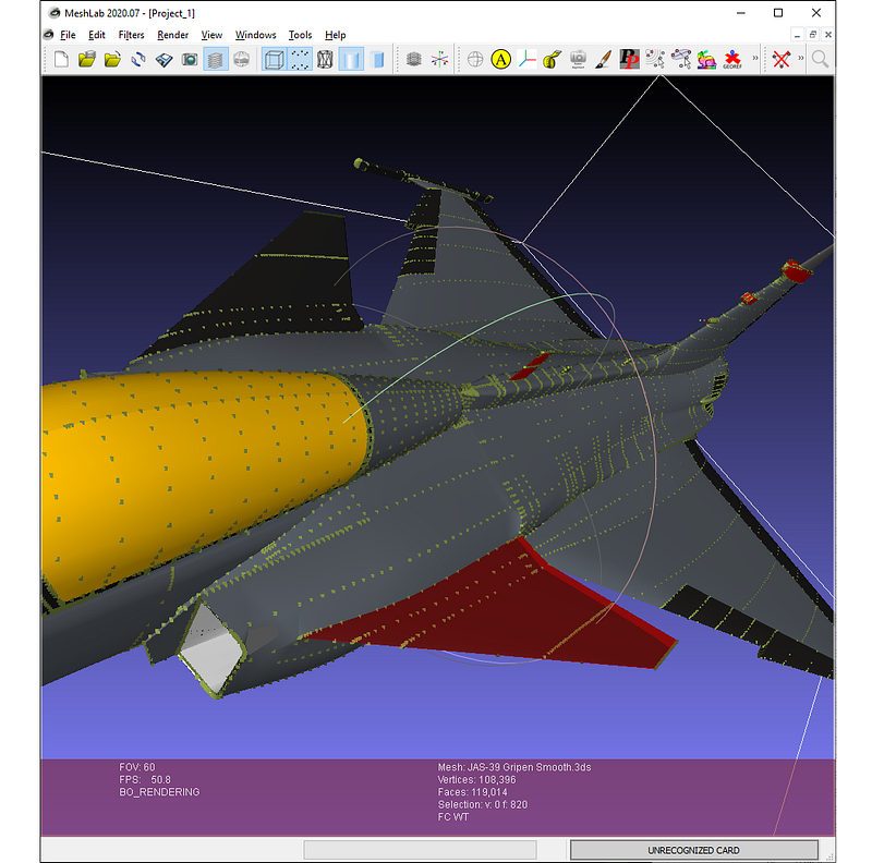
The first thing you will need to do is to look for is a 3D model in *.stl format (STereoLithography) that best represents the external geometry of the plane or air vehicle, like this example of a Saab 39 Gripen.
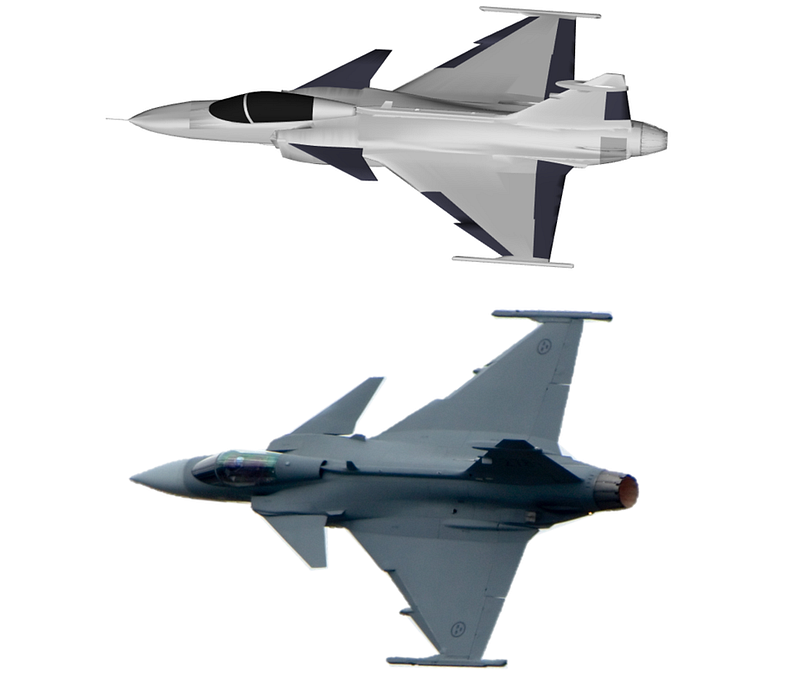
There is a wide variety of web pages where you can find an infinity of 3D models to download for free. I recommend you to have a look at the following websites where you will surely find the 3D model you are looking for:
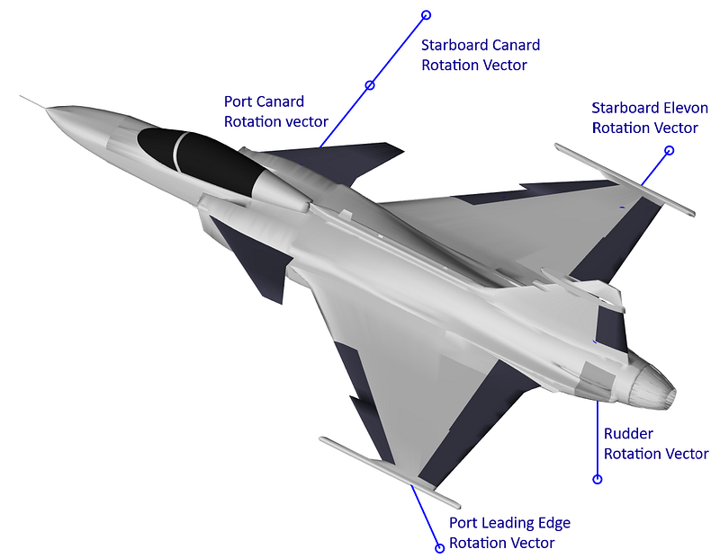
As our 3D animation tool will also allow animating the moving parts of the aircraft, we will have to separate the 3D model into two sets of parts/submodels: the rigid parts that are solidly attached to the main body (fuselage, wings, cockpit, etc.), and set of parts that can move and/or rotate with respect to the main body (flight control surfaces, landing gear, etc.).
In the case of the Saab Gripen 3D model, the moving parts set will be composed by:
- Canards (port/starboard)
- Flaperons (port/starboard)
- Leading Edge Flaps (port/starboard)
- Rudder
You can use any 3D editing tool to split the model’s moveable flight control surfaces, I personally like MeshLab, since it’s easy to use, and above all, it's completely free.
Step-2: Adapt the 3D Model to MATLAB’s Environment
Once you have separated the parts of the model into different *.stl files, we can start programming our script to load the *.stl file and generate a *.mat data file with the minimum relevant information to animate the moveable parts. This step is preferred because in Matlab it’s always faster to load data from a *.mat file than to read it from an ASCII or binary file (like the *.stl file).
To read the *.stl files in MATLAB you will need first to download the stlTools package from MATLAB’s file exchange web. Once you have downloaded the package, we can go straight to the coding business.
We will start adding the stlTools package’s path, defining the name of the *.mat output file containing the models’ data structure Model3D, and finally, we will define the properties of those *.stl files which are part of the aircraft’s rigid body geometry and those which are moveable surfaces.
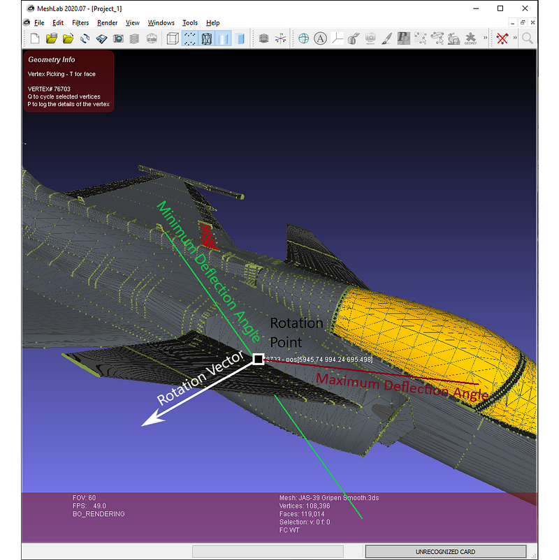
Each one of the model’s moveable surfaces requires you to define three important properties (the first two can be easily obtained using a 3D editing tool, i.e. MeshLab):
- Rotation Point: pivot point coordinates
- Rotation Vector: this parameter defines the flight control surface’s hinge direction
- Surface’s Maximum and Minimum Deflection Angles: a vector defining the movement limits.
After all of these properties definitions, we will read the *.stl files and save the vertex and faces information into the Model3D structure, along with the previously defined properties.
Now, we just have to save the Model3D structure in a mat file and plot all the model’s parts along with the moveable surfaces’ hinge line to check that everything looks fine.
At this point, we have finished our pre-processing script and we already have the MAT file containing the 3D model information, so we are ready for the next step, building the animation function.
Step-3: Build the Animation Function
Before we go further into the coding details, first I will brief you about two important Matlab’s built-in functions that we will use extensively, hgtransformand makehgtform.
We will use these built-in functions to apply translation and rotation transformations to the different parts of our 3D model in a straightforward way, with just two lines of code.
In Matlab, graphical objects like lines, surfaces, and patches can be grouped to share a common parent defining a set of spatial transformations (translation, scaling, and rotation) that apply to every child.
The transformation group handle is created using the hgtransform function, and the group association is performed via the ‘Parent’ property of the graphical objects. Here there is a simple example:
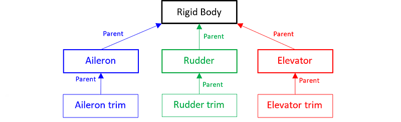
Right now you might be wondering, what’s the advantage of all of this? Well, imagine a Beech G36 Bonanza, an airplane with two ailerons, two elevators, and a rudder control surface.
Each one of the main control surfaces has a trim tab to alleviate the pilot’s control column forces in trimmed conditions. These trim tabs rotate around the hinge line located in the control surface, and this last one also rotates around its hinge line which solidary with the aircraft structure.
If we had to simulate the movement of the trim tabs, we would need to perform one translation and one rotation transformation over each individual part to respect the kinematic linkage between the control surfaces and the trim tabs.
However, we can do this in a much easier way using the hgtransform and makehgtform functions. Instead of applying individual transformations (translation and rotation) to each one of the surfaces, we could group them together into a parent transformation object recursively, to then just apply a single transformation to move all of them using two operations while fulfilling the kinematic rigid body conditions. This is the biggest advantage of this method.
The grouping or ‘parent’ strategy we would follow to solve this problem is depicted in the figure below.
Now that we have seen how graphical object groups work and how to apply transformations to them in an efficient way, we are ready to code the 3D animation function.
In this case, we will use the Saab Gripen 3D model we already prepared in Step-1 and Step-2, so we have to consider as inputs five different deflection angles for the flight control surfaces (symmetric canard, port, and starboard flaperons deflection, symmetric leading edges, and the rudder), the standard flight mechanic variables, and some auxiliary parameters that we will use to configure the video of the animation.
Remember that if your 3D model has more control surfaces than those of the Saab Gripen, you have to add them as additional inputs to the visualization function.
After defining the function’s interface, we will proceed to load the mat file containing the information of the model’s parts and initialize the video handle using the function (if we have selected to save the animation)
In a posterior step, we will open a new figure window with blank axes to then define the transformation groups that we are going to use to animate the graphical objects.
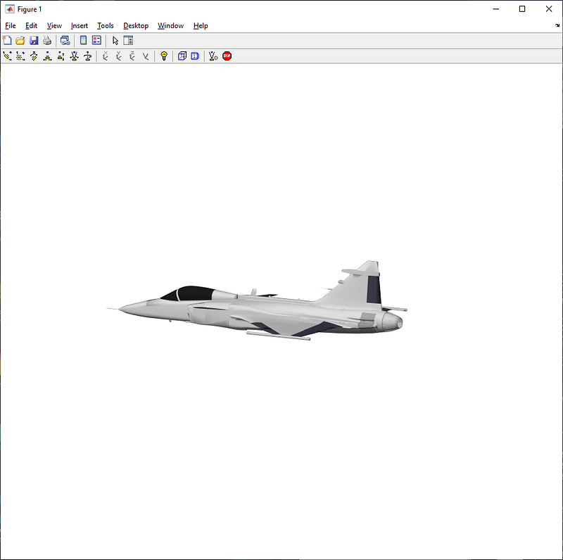
At this point, we are ready to start plotting our aircraft. First, we will plot the rigid body parts using the patch function and we will assign all of them to the parent (). Then we will continue plotting the moveable flight control surfaces and setting up the camera and lighting properties of the axis.
This is the look of the figure we have just plotted with a render of our 3D model. It looks good, isn't it?
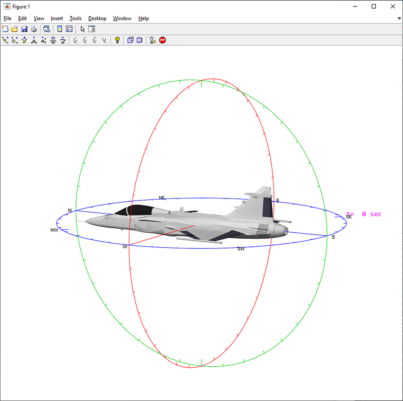
In the next step, we will plot additional visual references around the aircraft that will help us later to better visualize the movement of the aircraft and the variation of the Euler angles (heading, pitch, and bank angle). Attached to these references we will also display the current value of the most relevant flight parameters.
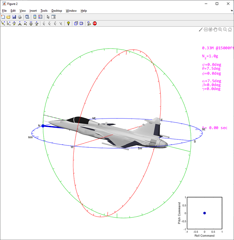
Now there are only two objects left to plot, the aircraft’s speed vector and the pilot stick inputs cross plot.
Now we have all the building blocks displayed in the figure, so we can proceed to animate the 3D model, frame by frame. The main steps we will follow in each frame are:
- Update the circles and lines representing the Euler angles
- Update the rigid parts’ transformation group
- Update the controls’ transformation group
- Update the aerodynamic speed vector
- Update the text handles with the current value of each one of the flight parameters represented in the figure
- Modify the aircraft’s color if it departs from controlled flight
- Modify the flight control surfaces’ color if they reach their maximum deflection angle (position saturation)
- Pause the loop if required to grant the animation is displayed in real-time
- Get the figure’s frame and add it to the movie file.
Here it’s the code snippet of the animation loop:
At this point, I bet you are eager to see an example of the animations that you can obtain with this tool, so let’s go for it!
What about a breakaway maneuver?

Maybe a rapid-rolling?

Or perhaps a scissors maneuver?
What I really like about these animations is that you can see at a glance the pilot’s stick position, the value of the main flight parameters, how the aircraft’s flight control surfaces move, and how the aerodynamic speed vector evolves during the maneuver.
With this kind of representation, even a non-expert in flight dynamics can comprehend what’s going on in a very complex maneuver. A video is worth a thousand time-histories, don’t you think so?
All You Are Looking for Is Here
I have collected all the previous code and examples in this Github repository. You will find in this repository a good suite of example maneuvers, as well as the last updated version of the animation function.
Takeaways
Now you have the knowledge, you know how the tool works, what are the building blocks, and how to modify them. So go play around with the code, and modify it as you wish for your own applications. The possibilities are endless.
Get that “wow” effect in your presentations with the videos you can record with this tool.
I hope you enjoy it, buddy.


