Adaptive Control (Part I) — Hypersonics and the MIT Rule

Introducing the algorithm that ruled the adaptive flight control system of the first manned hypersonic aircraft, the North American X-15.

We live in a world where control engineering is more important than ever.

In the last 10 years, we have seen how cars are able to drive autonomously, how the cost to access space has drastically decreased thanks to reusable rockets that can re-enter the atmosphere and land vertically, and how airplanes can operate without human intervention at all.

None of these incredible breakthroughs would have been possible without modern control systems. Practically every aspect of our day-to-day life is affected by some type of control algorithm.

Within the wide spectrum of the existing control techniques, there is a very special one called Adaptive Control, which has a unique capability, self-learning.

Just like our brain does, an adaptive controller has a sort of plasticity, as it can modify itself on the fly based on current and previous experiences.

If you are curious to know more about Adaptive Control, I’m sure you will enjoy this piece, the first one of a divulgation series where you will learn many of the basic concepts and methods of this thrilling field of Control Theory.

As in every good story, we will start from the very beginning of it all.

So we will time-travel to the early 60s, to the era of the Space Race and the firsts hypersonic manned flights, to introduce one of the most simple adaptation laws developed in the early days of Adaptive Control Theory: the famous “MIT rule”.

The MIT Rule: Adaptation via Gradient-Descent Optimization

The MIT rule was originally proposed by Osborn, Whitaker, and Kezer in a paper presented in the Institute of the Aerospace Science (today’s AIAA) back in 1961 under the title “New developments in the design of model reference adaptive control systems”.

It provided a very simple solution to the Model Reference Adaptive Control (MRAC) problem:

How to update the controller’s parameters to drive the response of the plant (vehicle) as close as possible to that of a stable reference system, which is considered optimal from the handling qualities’ point of view?

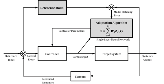
The authors of the MIT rule proposed to update the controller’s parameters θ via the minimization of a parametric error function E(θ) using a gradient descent adaptation law.

Just like when you throw a marble in a basin, the MIT rule would be like the gravity force that pushes the marble down the slope to the lowest point of the basin, where the marble’s energy (if it stops) is minimum. This is the basic working principle of the MIT rule.

The parametric error function E(θ) to be minimized in this case is usually defined as:

Where e(θ) represents a scalar model error, defined as the difference between the measured dynamics of the controlled vehicle and those of the reference system.

Using the gradient-descent optimization algorithm, the adaptation law is obtained by setting the time-derivative of the control parameter (dθ/dt) to be proportional to the negative gradient of the error function E(θ), yielding:

Where the proportional constant γ is a design parameter that defines the adaptive gain.

The previous equation represents the original mathematical formulation of the MIT rule, but there is also another variation that does not require the computation of the gradient (it only requires to know its sign):

As you can see, the MIT rule and its variations are all really simple in essence, so you might be thinking it was not a great “Eureka” idea, don’t you?

But the truth is that it really marked a watershed in the adaptive control history, as it provided impressive results in many of the early applications of the MRAC architectures.

One of the most famous applications of the MIT rule can be found in the history books of the firsts hypersonic research programs.

A Sweet Marriage to Rule the Hypersonics: the MRAC and the MIT Rule

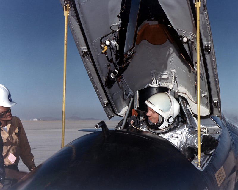
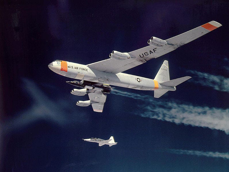
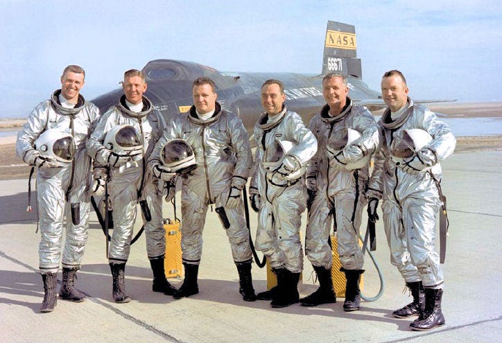
During the thrilling days of the Space Race, North American Aviation and Honeywell engineers were running against the clock to develop and flight-test a new type of manned aircraft. One that would explore the mysteries of hypersonic flight, the North American X-15.

This engineering marvel was born as part of NASA’s X-Plane program in close collaboration with the US Air Force. It was designed as a hypersonic research vehicle to explore the flight conditions that a space vehicle would face during its re-entry to Earth.

It was an era where the physics of hypersonics was still to be uncovered.

The first two prototypes of the X-15, the X-15–1 and the X-15–2, were equipped with a flight control system with different fixed-gain settings that could be selected by the pilot depending on the flight phase.

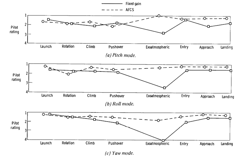
However, although in general, the fixed-gain control system provided adequate handling qualities in slow time-varying flight conditions, X-15’s pilots reported excessive workload at the cockpit during ballistic flights (weightlessness) and reentries.

The issues were related to the continuous corrections pilots had to make to deal with the poor handling qualities provided by the fixed-gain controller in fast time-varying flight conditions.

The handling quality degradation originated transitory oscillations in the pitch and yaw axis that usually appeared during the re-entry phase, while the vehicle was transiting from the ballistic to the atmospheric flight.

All of these issues made it difficult to accurately steer the vehicle in one of the most critical flight phases, the re-entry phase, and required the pilot to focus all of his senses around the control tasks.

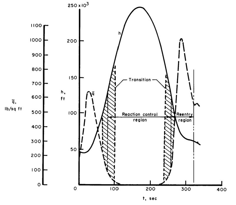
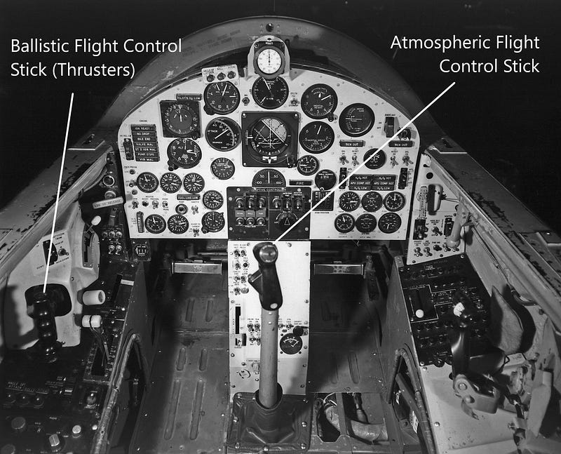
Moreover, during the transition phases where the vehicle entered or exited the ballistic flight (at around 125,000ft, where the dynamic pressure is typically 100lb/ft2), the pilot’s workload increased, even more, when he had to manually switch from the aerodynamic-control mode to the ballistic-control mode and vice versa.

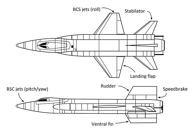
The ballistic-control mode of the X-15–1 and X-15–2 had an independent flight control stick from the aerodynamic-control mode and used reaction thrusters located at the nose and wingtips of the vehicle to provide pitching, yawing and rolling momentum.

All of the fixed-gain control system’s deficiencies paved the way for the development of many relatively new adaptive control technologies.

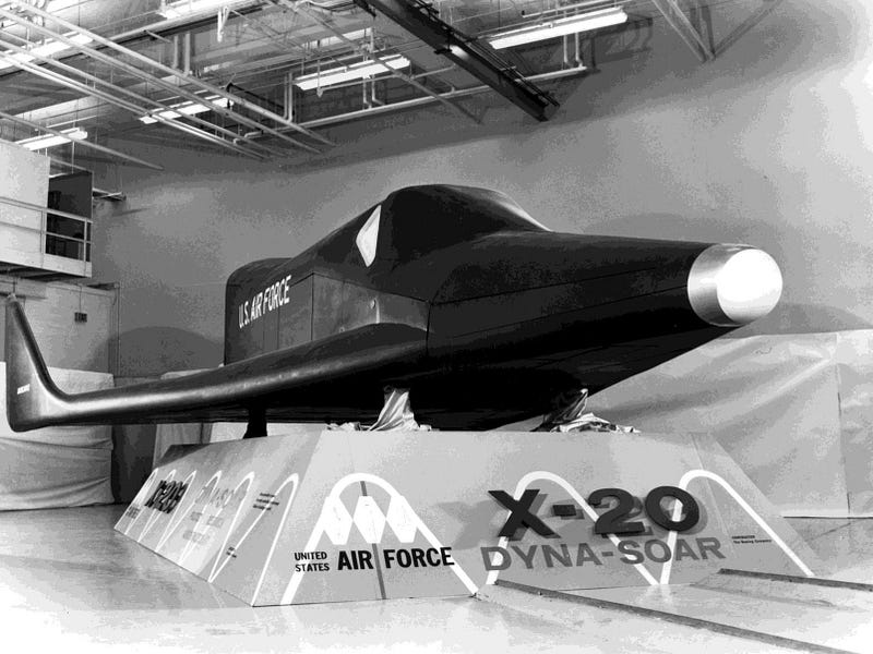
Circa 1961, Honeywell, the company that was in charge of the X-15’s flight control system development, saw the opportunity to test in the X-15 a new adaptive flight control hardware originally intended to be integrated into the X-20 Dyna-Soar prototype (the X-20 program and its MH-90 adaptive flight control system were prematurely canceled on December 10, 1963).

This new adaptive controller, whose official name in the X-15 program was the MH-96 AFCS (Adaptive Flight Control System), was a rate command, model-following controller, with a single scalar adaptive gain, which was based on an MRAC architecture that used the MIT rule for its adaptation law.

The X-15–3, the third prototype, was the only prototype equipped with the new MH-96 adaptive control system, and then it was one of the first aircraft in the history of aeronautics to feature an adaptive controller.

The controller’s architecture for the pitch axis was similar to that shown in Figure 4, with the reference system defined by a first-order low pass filter with a time constant (τ) of 0.5sec.

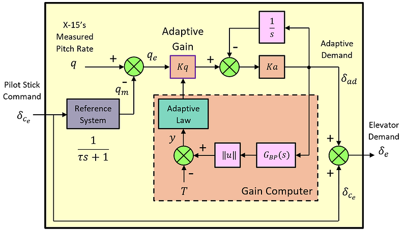
The main objective of this architecture was to make the controller operate always with the adaptive gain (denoted by Kq in Figure 9) at the highest possible value, but without triggering unacceptable high-frequency instabilities.

In this way, the adaptive controller will drive the vehicle dynamics close to the reference model as fast as possible.

The adaptive gain’s upper limit, which defines the thin line between a stable and an unstable system, was an unknown parameter that depends on the flight condition and on the actuators’ dynamics.

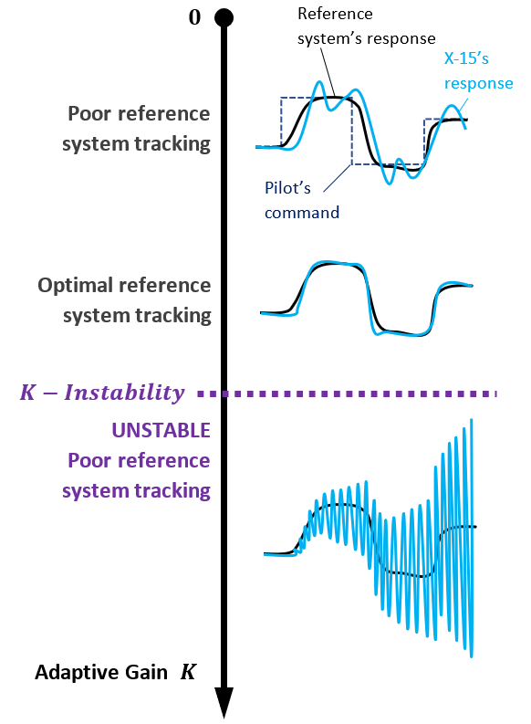
But flying at the edge of instability was indeed the objective of the MH-96 adaptive control system, as it was at this point where the handling qualities of the X-15 would better match those of the reference model.

This idea is paramount to understand how the MIT law was applied in the MH-96 controller.

At the edge of instability, the adaptive demand path of the MH-96 controller would exhibit a limit cycle oscillation with a frequency very close to the natural frequency of the servo-actuator loop (90rad/s for the elevons and 70rad/s for the rudder).

Knowing this effect, then it was evident for Honeywell’s control engineers they had to select an error function E(K) of the form:

Where T is a threshold between acceptable and unacceptable oscillation’s amplitude, K is the adaptive gain, and ||u(K)||is the amplitude of the adaptive demand component around a frequency bandwidth centered at the natural frequency of the servo-actuator loop.

Then, applying the MIT rule to minimize this error, they obtained the following adaptation law for the K gain (the actual adaptation law included additional rate limits and saturation):

Considering that:

The MIT rule finally yields:

Observe that if the amplitude of the oscillations is lower than the threshold T, then the adaptation gain K increases, and vice versa.

The value of the adaptive gain K was also used in the MH-96 adaptive system to perform an automatic blending between the aerodynamic control mode and the ballistic control mode.

For small values of the gain K, the ballistic-control mode was automatically disengaged, but once the value of the gain K exceeded a switch-on threshold (indicating a decrease in the aerodynamic control power) the reaction control thrusters were engaged back again, providing a nearly transparent control transition during the ascend and reentry.

Moreover, as the reference system was kept constant through the whole flight envelope, the MH-96 proved to provide a homogeneous response and good handling qualities in all the control axis.

With this adaptation law, the X-15–3 and its MH-96 adaptive flight control system achieved superior performances compared to their fixed-gain counterparts (X-15–1 and X-15–2).

A very good summary of the pilot’s feedback on the MH-96 adaptive system can be found in the following extract from this NASA’s report:

“The true superiority of the X-15 AFCS was that it unburdened the pilot. The airplane was stable at any dynamic pressure and at any angle of attack. The AFCS inspired confidence and allowed the pilot to spend time cross-checking flight instruments, checking subsystems, and “sightseeing.”” — Pilot observations from Experience with the X-15 Adaptive Flight Control System report.

What’s Next?

In the next chapter of this series, we will learn how to build a simplified Simulink model of the X-15’s MH-96 AFCS.

You know what they say, an image is worth a thousand words. But in control engineering, I would rather say “a Simulink model is worth a thousand equations”.

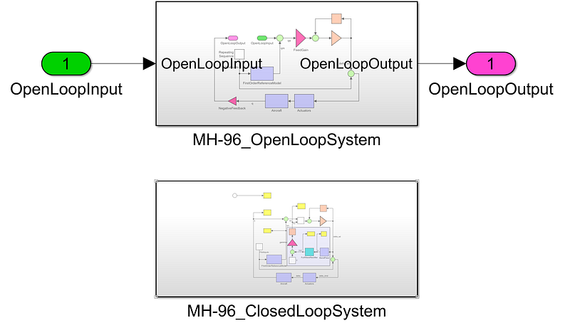
So given the fairly simple architecture of the MH-96 control system, you will see how it’s straightforward to implement it in a Simulink model, to have a firsthand view of the MIT rule’s performance in a real-life example.

See you in the next chapter!

References

[1] Iven M.Y. Mareels, Brian D.O. Anderson, Robert R. Bitmead, Marc Bodson, Shankar S. Sastry, Revisiting the Mit Rule for Adaptive Control, IFAC Proceedings Volumes, Volume 20, Issue 2, 1987, Pages 161–166, ISSN 1474–6670

[2] NASA Armstrong Fact Sheet: X-15 Hypersonic Research Program

[3] Orr J.S., Statler I.C., Barshi I. (2015) The X-15 3–65 Accident: An Aircraft Systems and Flight Control Perspective. In: Sgobba T., Rongier I. (eds) Space Safety is No Accident. Springer, Cham.

[4] NASA Technical Report: The X-20 Flight Control System Development

[5] Dydek, Zachary, Anuradha Annaswamy, and Eugene Lavretsky. “Adaptive Control and the NASA X-15–3 Flight Revisited.” IEEE Control Systems Magazine 30.3 (2010): 32–48. Web.© 2010 IEEE.

[6] NASA Technical Report. Experience With the X-15 Adaptive Flight Control System.

Rodney Rodríguez Robles is an aerospace engineer, cyclist, blogger, and cutting edge technology advocate, living a dream in the aerospace industry he only dreamed of as a kid. He talks about coding, the history of aeronautics, control engineering, rocket science, and all the technology that is making your day by day easier.

Please check me out on the following social networks as well, I would love to hear from you! — LinkedIn, Twitter.