A Deep Dive into the Code of the Visual Transformer (ViT) Model

Breaking down the HuggingFace ViT Implementation

Vision Transformer (ViT) stands as a remarkable milestone in the evolution of computer vision. ViT challenges the conventional wisdom that images are best processed through convolutional layers, proving that sequence-based attention mechanisms can effectively capture the intricate patterns, context, and semantics present in images. By breaking down images into manageable patches and leveraging self-attention, ViT captures both local and global relationships, enabling it to excel in diverse vision tasks, from image classification to object detection and beyond. In this article, we are going to break down how ViT for classification works under the hood.

Introduction

The core idea of ViT is to treat an image as a sequence of fixed-size patches, which are then flattened and converted into 1D vectors. These patches are subsequently processed by a transformer encoder, which enables the model to capture global context and dependencies across the entire image. By dividing the image into patches, ViT effectively reduces the computational complexity of handling large images while retaining the ability to model complex spatial interactions.

First of all, we import the ViT model for classification from hugging face transformers library:

from transformers import ViTForImageClassification
import torch
import numpy as np

model = ViTForImageClassification.from_pretrained("google/vit-base-patch16-224")

patch16–224 indicates that the model accepts images of size 224x224 and each patch has width and hight of 16 pixels.

This is what the model architecture looks like:

ViTForImageClassification(
  (vit): ViTModel(
    (embeddings): ViTEmbeddings(
      (patch_embeddings): PatchEmbeddings(
        (projection): Conv2d(3, 768, kernel_size=(16, 16), stride=(16, 16))
      )
      (dropout): Dropout(p=0.0, inplace=False)
    )
    (encoder): ViTEncoder(
      (layer): ModuleList(
        (0): ViTLayer(
          (attention): ViTAttention(
            (attention): ViTSelfAttention(
              (query): Linear(in_features=768, out_features=768, bias=True)
              (key): Linear(in_features=768, out_features=768, bias=True)
              (value): Linear(in_features=768, out_features=768, bias=True)
              (dropout): Dropout(p=0.0, inplace=False)
            )
            (output): ViTSelfOutput(
              (dense): Linear(in_features=768, out_features=768, bias=True)
              (dropout): Dropout(p=0.0, inplace=False)
            )
          )
          (intermediate): ViTIntermediate(
            (dense): Linear(in_features=768, out_features=3072, bias=True)
          )
          (output): ViTOutput(
            (dense): Linear(in_features=3072, out_features=768, bias=True)
            (dropout): Dropout(p=0.0, inplace=False)
          )
          (layernorm_before): LayerNorm((768,), eps=1e-12, elementwise_affine=True)
          (layernorm_after): LayerNorm((768,), eps=1e-12, elementwise_affine=True)
        )
        
        .......

        (11): ViTLayer(
          (attention): ViTAttention(
            (attention): ViTSelfAttention(
              (query): Linear(in_features=768, out_features=768, bias=True)
              (key): Linear(in_features=768, out_features=768, bias=True)
              (value): Linear(in_features=768, out_features=768, bias=True)
              (dropout): Dropout(p=0.0, inplace=False)
            )
            (output): ViTSelfOutput(
              (dense): Linear(in_features=768, out_features=768, bias=True)
              (dropout): Dropout(p=0.0, inplace=False)
            )
          )
          (intermediate): ViTIntermediate(
            (dense): Linear(in_features=768, out_features=3072, bias=True)
          )
          (output): ViTOutput(
            (dense): Linear(in_features=3072, out_features=768, bias=True)
            (dropout): Dropout(p=0.0, inplace=False)
          )
          (layernorm_before): LayerNorm((768,), eps=1e-12, elementwise_affine=True)
          (layernorm_after): LayerNorm((768,), eps=1e-12, elementwise_affine=True)
        )
      )
    )
    (layernorm): LayerNorm((768,), eps=1e-12, elementwise_affine=True)
  )
  (classifier): Linear(in_features=768, out_features=1000, bias=True)
)

Embeddings

Patch Embedding

Transformation of the image into patches is performed using a Conv2D layer. As we know, Conv2D layer does a 2-dimensional convolutional operations on input data to learn features and patterns from images. In this case though Conv2D layer is used to divide the image into NxN number of patches by using the stride parameter. Stride determines the step size at which the filter slides over the input data. In this case, because our images are 224x224 and the patch is of size 16, meaning that there are 224/16 = 14 patches in each dimension, if we choose stride=16 we effectively separate our image in 14 non-overlapping patches.

To be visual and assuming an image of shape 4x4 with and stride of 2:

So for example, the first & the second patches are going to be :

proj = model.vit.embeddings.patch_embeddings.projection
torch.allclose(torch.sum(image[0, :, 0:16, 0:16] * w[0]) + b[0],
               proj(image)[0][0][0, 0], atol=1e-6)
# True


torch.allclose(torch.sum(image[0, :, 16:32, 0:16] * w[0]) + b[0],
                 proj(image)[0][0][1, 0], atol=1e-6)

# True

The pattern is clear — to compute each patch we skip 16 pixels to get non-overlapping patches. If we do this operation for the entire image we end up with 1 x 14 x 14 tensor where each patch is represented by one number computed using the first filter of Conv2D. However, there are 768 filters which means that at the end we get a 768 x 14 x 14 dimensional tensor. So now we effectively have for each patch a 768 dimensional representation, that is our patch embedding. We also flatten and transpose the tensor, thus the embedding shape becomes [batch_size, 196, 768] where the second dimension is flattened 14 x 14 = 196 and we effectively have a sequence of 196 patches with embedding size of 768.

embeddings = model.vit.embeddings.patch_embeddings.projection(image)
# shape (batch_size, 196, 768)
embeddings = embeddings.flatten(2).transpose(1, 2)

If we want to reproduce the layer entirely from scratch, this is the code:

batch_size = 1 
F = 768 # number of filters
H1 = 14 # output dimension hight - 224/16
W1 = 14 # output dimension width - 224/16
stride = 16
HH = 16 # patch hight
WW = 16 # patch width
w = model.vit.embeddings.patch_embeddings.projection.weight
b = model.vit.embeddings.patch_embeddings.projection.bias

out = np.zeros((N, F, H1, W1))
chunks = []
for n in range(batch_size):
    for f in range(F):
        for i in range(H1):
            for j in range(W1):
                # perform convolution operation
                out[n, f, i, j] = torch.sum( image[n, :, i*stride:i*stride+HH, j*stride : j*stride + WW] * w[f] ) + b[f]
                
np.allclose(out[0], embeddings[0].detach().numpy(), atol=1e-5)
# True

Now, if you are familiar with the Language Transformer (check it out here if needed) you should recall the [CLS] token, whose representation serves as a condensed and informative summary of the entire text, enabling the model to make accurate predictions based on the extracted features from the transformer encoder. Also in ViT we have the [CLS] token that has the same function as for text, and it’s appended to the representation computed above.

[CLS] token is a parameter that we are going to learn using back-propagation:

cls_token = nn.Parameter(torch.randn(1, 1, 768))
cls_tokens = cls_token.expand(batch_size, -1, -1)
# append [CLS] token
embeddings = torch.cat((cls_tokens, embeddings), dim=1)

Positional Embedding

Just like in Language Transformer, to preserve the positional information of the patches, ViT includes positional embeddings. Positional embeddings help the model understand the spatial relationships between different patches, enabling it to capture the image’s structure. Positional embedding is a Tensor of the same shape of the embeddings with [CLS] token compute before, i.e., [batch_size, 197, 768]

embeddings = embeddings + model.vit.embeddings.position_embeddings

Dropout

Patch embedding is followed by a Dropout layer. In dropout we replace with zero some of the values with certain dropout probability. Dropout helps to reduce overfitting as we randomly block signals from certain neurons so the network needs to find other paths to reduce the loss function, and thus it learns how to generalize better instead of relying on certain paths. We can also see dropout as a kind of models ensemble technique as during training at each step we randomly deactivate certain neurons ending up with “different” networks which we eventually ensemble during the evaluation time.

At the end of the Embeddings layer we have:

# compute the embedding
embeddings = model.vit.embeddings.patch_embeddings.projection(image)
embeddings = embeddings.flatten(2).transpose(1, 2)
# append [CLS] token
cls_token = model.vit.embeddings.cls_token
embeddings = torch.cat((cls_tokens, embeddings), dim=1)
# positional embedding
embeddings = embeddings + self.position_embeddings
# droput
embeddings = model.vit.embeddings.dropout(embeddings)

Encoder

ViT employs a stack of transformer encoder blocks, similar to those used in language models such as BERT. Each encoder block consists of multi-head self-attention and feed-forward neural networks. The self-attention mechanism enables the model to capture relationships between different patches, while the feed-forward neural networks perform non-linear transformations.

Specifically, each layer is composed of Self-Attention, Intermediate and Output modules.

(0): ViTLayer(
  (attention): ViTAttention(
    (attention): ViTSelfAttention(
      (query): Linear(in_features=768, out_features=768, bias=True)
      (key): Linear(in_features=768, out_features=768, bias=True)
      (value): Linear(in_features=768, out_features=768, bias=True)
      (dropout): Dropout(p=0.0, inplace=False)
    )
    (output): ViTSelfOutput(
      (dense): Linear(in_features=768, out_features=768, bias=True)
      (dropout): Dropout(p=0.0, inplace=False)
    )
  )
  (intermediate): ViTIntermediate(
    (dense): Linear(in_features=768, out_features=3072, bias=True)
  )
  (output): ViTOutput(
    (dense): Linear(in_features=3072, out_features=768, bias=True)
    (dropout): Dropout(p=0.0, inplace=False)
  )
  (layernorm_before): LayerNorm((768,), eps=1e-12, elementwise_affine=True)
  (layernorm_after): LayerNorm((768,), eps=1e-12, elementwise_affine=True)
)

Self-Attention

Self-attention is a pivotal mechanism within the Vision Transformer (ViT) model that enables it to capture relationships and dependencies between different patches in an image. It plays a crucial role in extracting contextual information and understanding long and short-range interactions among the patches.

Each patch is associated with three vectors: Key, Query, and Value. These vectors are learned through linear transformations of the original patch embeddings. The Key vector represents information from the current patches, the Query vector is used to ask questions about other patches, and the Value vector holds the information that is relevant to other patches.

As we have already computed the embeddings in the previous section, we compute the Key, Query and Value projecting the embeddings with the Key, Query and Value matrices:

import math 
import torch.nn as nn

torch.manual_seed(0)

hidden_size = 768
num_attention_heads = 12
attention_head_size = hidden_size // num_attention_heads # 64

hidden_states = embeddings

# apply LayerNorm to the embeddings
hidden_states = model.vit.encoder.layer[0].layernorm_before(hidden_states)

# take first layer of the Transformer
layer_0 = model.vit.encoder.layer[0]

# shape (768, 64) 
key_matrix = layer_0.attention.attention.key.weight.T[:, :attention_head_size]
key_bias = layer_0.attention.attention.key.bias[:attention_head_size]

query_matrix = layer_0.attention.attention.query.weight.T[:, :attention_head_size] 
query_bias = layer_0.attention.attention.query.bias[:attention_head_size]

value_matrix = layer_0.attention.attention.value.weight.T[:, :attention_head_size]
value_bias = layer_0.attention.attention.value.bias[:attention_head_size]

# compute key, query and value for the first head attention
# all of shape (b_size, 197, 64)
key_1head = hidden_states @ key_matrix + key_bias
query_1head = hidden_states @ query_matrix + query_bias
value_1head = hidden_states @ value_matrix + value_bias

Note that we skipped the LayerNorm operation, that we will cover later.

For each Query vector, attention scores are computed by measuring the compatibility or similarity between the Query and Key vectors of all other patches. This is done through a dot product operation and then applying the Softmax function to get normalized attention scores with the shape [b_size, 197, 197]. The attention matrix is square because all patches attend to each other, and this is why it’s called self-attention. These scores indicate how much focus or attention should be placed on each patch when processing the query patch. Because new embedding for the next layer of each patch is derived based on the attention scores and the values of all other patches, we get a contextual embedding for each patch as its derived based on all other patches in the image.

To clarify this further, recall that at the beginning we split the image into patches using the Conv2D layer to get a 768-dimensional embedding vector for each patch - these embedding are independent as there was no interaction (no overlap) between the patches. However, in the transformer layers the patches embeddings get mixed becoming a function of the embeddings of other patches. For example, the embedding in the first layer is:

# shape (b_size, 197, 197)
# compute the attention scores by dot product of query and key
attention_scores_1head = torch.matmul(query_1head, key_1head.transpose(-1, -2))

attention_scores_1head = attention_scores_1head / math.sqrt(attention_head_size)
attention_probs_1head = nn.functional.softmax(attention_scores_1head, dim=-1)

# contextualized embedding for this layer
context_layer_1head = torch.matmul(attention_probs_1head, value_1head)

If we zoom in and look at the first patch:

patch_n = 1
# shape (, 197)
print(attention_probs_1head[0, patch_n])
[2.4195e-01, 7.3293e-01, ..,
        2.6689e-06, 4.6498e-05, 1.1380e-04, 5.1591e-06, 2.1265e-05],
     

the new embeddings for it (token indexed at 0 is [CLS] token) is a combination of embeddings of different patches with most attention on the first patch itself (0.73), [CLS] token (0.24) and the remaining on all other patches. But this is not always the case. Indeed, in next layers the first patch might pay more attention to patches around it instead of the patch itself and [CLS] token or even to patches very far away — this depends on what the model thinks is useful to solve a certain task.

Also, you might have noticed that I selected only the first 64 columns from the weight matrices of query, key and value. These first 64 columns represent the first attention head, but actually there are 12 of them (in this model size). Each of these attention heads creates different representation of patches. Indeed, if we look at the third attention head for the first patch we can see that the first patch pays most attention (0.26) at the second patch rather than to itself like in the first attention head.

# shape (, 197)
[2.6356e-01, 1.2783e-03, 2.6888e-01, ... , 1.8458e-02]

Thus, different attention heads will capture different types of relations among patches helping the model to see things from different prospective.

To compute all these heads in parallel we do as follows:

def transpose_for_scores(x: torch.Tensor) -> torch.Tensor:
    new_x_shape = x.size()[:-1] + (num_attention_heads, attention_head_size)
    x = x.view(new_x_shape)
    return x.permute(0, 2, 1, 3)

mixed_query_layer = layer_0.attention.attention.query(hidden_states)

key_layer = transpose_for_scores(layer_0.attention.attention.key(hidden_states))
value_layer = transpose_for_scores(layer_0.attention.attention.value(hidden_states))
query_layer = transpose_for_scores(mixed_query_layer)

# Take the dot product between "query" and "key" to get the raw attention scores.
attention_scores = torch.matmul(query_layer, key_layer.transpose(-1, -2))
attention_scores = attention_scores / math.sqrt(attention_head_size)

# Normalize the attention scores to probabilities.
attention_probs = nn.functional.softmax(attention_scores, dim=-1)

# This is actually dropping out entire tokens to attend to, which might
# seem a bit unusual, but is taken from the original Transformer paper.
attention_probs = layer_0.attention.attention.dropout(attention_probs)

context_layer = torch.matmul(attention_probs, value_layer)

context_layer = context_layer.permute(0, 2, 1, 3).contiguous()
new_context_layer_shape = context_layer.size()[:-2] + (hidden_size,)
context_layer = context_layer.view(new_context_layer_shape)

After applying self-attention we apply another projection layer and Dropout — and here we go, we got through the self-attention layer!

output_weight = layer_0.attention.output.dense.weight
output_bias = layer_0.attention.output.dense.bias

attention_output = context_layer @ output_weight.T + output_bias
attention_output = layer_0.attention.output.dropout(attention_output)

Ops, wait a second, I promised I would explain the LayerNorm operation.

Layer Normalization is a normalization technique used to enhance the training and performance of deep learning models. It addresses the problem of internal covariate shifts — during training, as the weights of the neural network change, the distribution of inputs to each layer can change significantly, making it difficult for the model to converge. Layer Normalization addresses this by ensuring that the inputs to each layer have a consistent mean and variance, stabilizing the learning process. It’s implemented by standardizing each patch embedding by its mean and standard deviation so that it has zero mean and unit variance. We then apply a trained weights and bias so it can be shifted to have a different mean and variance for the model to adapt automatically during training. Because we compute mean and standard deviation across different examples independently from the others, it is different from Batch Normalization where the normalization is across the batch dimension and thus depends on other examples in the batch.

Let’s take the first patch embedding:

first_patch_embed = embeddings[0][0]
# compute first patch mean
first_patch_mean = first_patch_embed.mean()
# compute first patch variance
first_patch_std = (first_patch_embed - first_patch_mean).pow(2).mean()
# standardize the first patch
first_patch_standardized = (first_patch_embed - first_patch_mean) / torch.sqrt(first_patch_std + 1e-12)
# apply trained weight and bias vectors
first_patch_norm = layer_0.layernorm_before.weight * first_patch_standardized + layer_0.layernorm_before.bias

Intermediate

Before the Intermediate class we perform another layer normalization and a residual connection. By now it should be clear why we want to apply another layer normalization — we need to normalize the contextual embeddings coming from the self-attention to improve convergence, but what is that other residual thing I mentioned you are probably wondering? Residual Connection is a critical component in deep neural networks that mitigates the challenges of training very deep architectures. As we increase the depth of a neural network by stacking more layers we bump into the problem of vanishing/exploding gradients, where in case of vanishing gradients the model is not able to learn anymore as the propagated gradients are close to zero and initial layers stop changing weights and improve (Check this article and this if you want to learn more about the vanishing gradient). Opposite problem with exploding gradients when the weights cannot stabilize because of extreme updates which eventually explode (go to infinity). Now, proper initialisation of weights and normalization helps to address this problem but what has been observed is even if the network becomes more stable, the performance decreases as the optimization is harder. Adding these residual connections helps to improve performance and the network becomes easier to optimize even if we keep increasing depth.

How is it implemented? Simple — we just add the original input to the transformed output after some transformations of the original input:

transformations = nn.Sequential([nn.Linear(), nn.ReLU(), nn.Linear()])
output = input + transformations(input)

Another key insight is that if the transformations of a residual connection learn to approximate the identity function, the addition of the input with the learned features will not have any effect. In fact, the network can learn to modify or refine the features if needed.

In our case the residual connection is the sum between the initial embeddings and the attention_output which are embeddings after all the transformations in the self-attention layer.

# first residual connection - NOTE the hidden_states are the 
# `embeddings` here
hidden_states = attention_output + hidden_states

# in ViT, layernorm is also applied after self-attention
layer_output = layer_0.layernorm_after(hidden_states)

In the Intermediate class we perform a linear projection and apply a non-linearity:

layer_output_intermediate = layer_0.intermediate.dense(layer_output)
layer_output_intermediate = layer_0.intermediate.intermediate_act_fn(layer_output_intermediate)

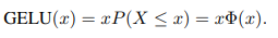
The non-linearity used in ViT is GeLU activation function. It is defined as the cumulative distribution function of the standard normal distribution:

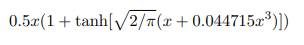
It is normally approximated with the following formula for faster calculations:

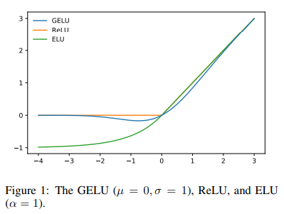
Looking at the graph below we can see that if ReLU, that is given by the formula max(input, 0), is monotonic, convex and linear in the positive domain, GeLU is non-monotonic, non-convex and non-linear in the positive domain and thus can approximate more easily complicated functions. Additionally, GeLU function is smooth — unlike the ReLU function, which is piecewise linear with a sharp transition at zero, GeLU provides a smooth transition across all values, making it more amenable to gradient-based optimization during training.

Output

The final bit remaining of the Encoder is the Output class. To compute it we already have all the elements we need — it is linear projection, Dropout and a residual connection:

# linear projection
output_dense = layer_0.output.dense(layer_output_intermediate)
# dropout
output_drop = layer_0.output.dropout(output_dense)
# residual connection - NOTE these hidden_states are computed in 
# Intermediate 
output_res = output_drop + hidden_states # shape (b_size, 197, 768)

Well, we went through the first layer ViT Layer, there are other 11 to go through and this is where the hard part comes …

Joking! We are actually done — all the other layers are exactly the same as the first, the only difference is that instead of starting from the embeddings like in the first layer the embeddings for the next layer are output_res we computed previously.

So the output after 12 layer of the encoder is:

torch.manual_seed(0)
# masking heads in a given layer
layer_head_mask = None
# output attention probabilities
output_attentions = False

embeddings = model.vit.embeddings(image)
hidden_states = embeddings
for l in range(12):
    hidden_states = model.vit.encoder.layer[l](hidden_states, layer_head_mask, output_attentions)[0]

output = model.vit.layernorm(sequence_output)

Pooler

Generally, in a Transformer model Pooler is a component used to aggregate information from the sequence of tokens embeddings after the transformer encoder blocks. Its role is to generate a fixed-size representation that captures the global context and summarizes the information extracted from the image patches, in case of ViT. The Pooler is essential for obtaining a compact and context-aware representation of the image, which can then be used for various downstream tasks such as image classification.

In this case Pooler is very simple — we take [CLS] token and use it as the compact and context-aware representation of the image.

pooled_output = output[:, 0, :] # shape (b_size, 768)

Classifier

Finally, we are ready to use the the pooled_output to classify the image. The classifier is a simple linear layer with output dimension equal to the number of classes:

logits = model.classifier(pooled_output) # shape (b_size, num_classes)

Conclusions

ViT fully revolutionized computer vision replacing Convolutional Neural Networks almost in every application, this is why it’s so important to understand how it works. Let’s not forget that the transformer architecture, which is the main component of ViT, originated in NLP, thus you should check out my previous article on BERT Transformer here. Hope you enjoyed this read, see you next time!

References

[1] https://github.com/huggingface/transformers [2] [2010.11929] An Image is Worth 16x16 Words: Transformers for Image Recognition at Scale (arxiv.org)