
Backpropagation and Vanishing Gradient Problem in RNN (Part 2)
How it is reduced in LSTM

In part 1 of this series, we went through back-propagation in an RNN model and explained both with formulas and showed numerically the vanishing gradient problem in RNN. In this article, we are going to explain how we can partially solve the vanishing gradient problem with LSTM even if it does not completely disappear and with very long sequences the problem still persists.
Motivation
As we have seen in part 1 of this series, vanilla RNN stores the temporal information in the hidden state which is updated at each time-step when new information is added, i.e., a new token in a sequence is processed. Because the hidden state is updated at every step, the old information is overwritten and the network forgets what it has seen in the past. To avoid this, we need a separate memory and a mechanism that decides what to write into it, given new information, what to delete from the past which will not be useful in the future and what to pass to the next state. LSTM does exactly that — it adds a memory cell that stores long-term information and has a gating mechanism that is used to decide what to forget from the past, add from the current input, and pass forward.
Forward propagation
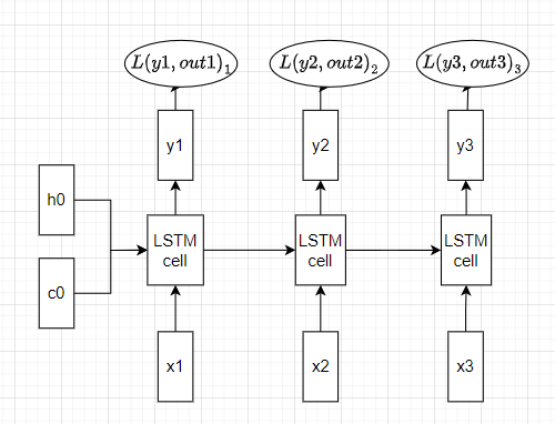
Let’s see how forward propagation through time is performed in an LSTM model. Given a sequence of N tokens and assuming we received a memory cell c(t-1) and a hidden state h(t-1) from the previous cell, at a time-step t we compute the gates to decide what to do with the new incoming information. First, let’s compute the activations:
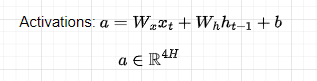
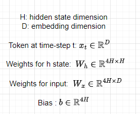
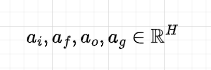
Remember that all the weights are shared across time-steps. The activations matrix is then split into 4 matrices, each of dimension H, and applying a sigmoid activation function to the first 3 and tanh to the last, we compute the gates:
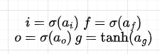
Note how all the gates are functions of the input and previous hidden state.
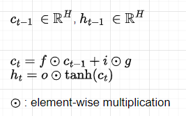
Finally, we compute the current memory cell state c(t) and hidden state h(t) that will be passed to the next step.
The gates values computed have the following functionalities:
- gate f: what information to forget from the previous memory cell c(t-1). Note that as we do element-wise multiplication (remember c(t-1) and h(t-1) are vectors) and f contains values between 0 and 1 due to the sigmoid activation function, it will cancel or reduce the information in c(t-1) when the values of f equal or closer to 0 and will maintain all or almost all the information when the values of f are equal or close to 1.
- gate g: can be interpreted as the memory cell update vector that is combined with the previous memory cell c(t-1) to compute the new memory cell c(t). Differently from other gates, a tanh function is applied to the activation a(g) which outputs a value between -1 and 1. This is to allow the cell memory state to both increase and decrease, as if we had a sigmoid activation, the elements of the memory cell could never decrease.
- gate i: what information to write from the memory cell update vector (gate g) to the previous memory cell c(t-1).
- gate o: what information to include in the new hidden state h(t)
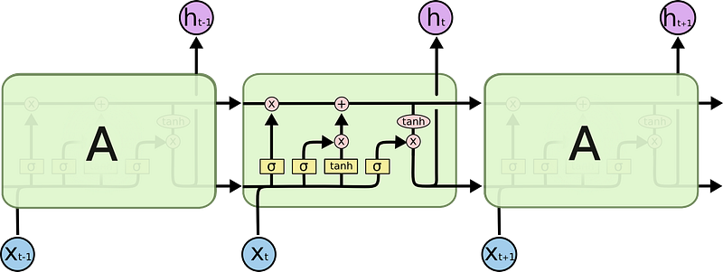
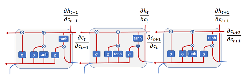
These gates are then combined, as illustrated in Figure 4 to compute the new memory cell c(t) and hidden state h(t). These new cells and hidden state are then passed to the next LSTM cell that repeats the same process again. All this process can be illustrated in the below diagram:
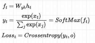
After that, for each hidden state, we compute the output and the loss:
In code:
def softmax(x, axis=2):
    p = np.exp(x - np.max(x, axis=axis,keepdims=True))
    return p / np.sum(p, axis=axis, keepdims=True)

def lstm_step_forward(x, prev_h, prev_c, Wx, Wh, b):

    next_h, next_c, cache = None, None, None

    h = x @ Wx + prev_h @ Wh + b
    assert h.shape[-1] % 4 == 0
    ai, af, ao, ag = np.array_split(h, 4, axis=-1)
    i = sigmoid(ai)
    f = sigmoid(af)
    o = sigmoid(ao)
    g = np.tanh(ag)

    next_c = f * prev_c + i * g
    next_h = o * np.tanh(next_c)

    cache = (x, next_h, prev_h, prev_c, Wx, Wh, h, np.tanh(next_c), i, f, o ,g)

    return next_h, next_c, cache


np.random.seed(232)

# N - Batch size
# D - Embeddding dimension
# V - Vocabulary size
# H - Hidden dimension
# T - timesteps
N, D, T, H, V = 2, 5, 3, 4, 4

x  = np.random.randn(N, T, D)
h0 = np.random.randn(N, H)
Wx = np.random.randn(D, H)
Wh = np.random.randn(H, H)
Wy = np.random.randn(H, V)
b  = np.random.randn(H)

y = np.random.randint(V, size=(N, T))
mask = np.ones((N, T))


all_cache = []
h = np.zeros((N, T, H))
next_c = np.zeros((N, H))

for t in range(T):
    xt = x[:, t , :]
    if t == 0:
        next_h, next_c, cache_s = lstm_step_forward(xt, h0, next_c, Wx, Wh, b)
        all_cache.append(cache_s)
    else:
        next_h, next_c, cache_s = lstm_step_forward(xt, next_h, next_c, Wx, Wh, b)
        all_cache.append(cache_s)

    h[:, t, :] = next_h

ft = h @ Wy
out = softmax(ft)
Backpropagation
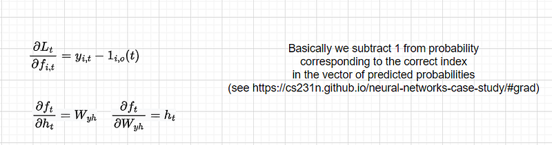
The formulas for back-propagation are a bit more involved than the ones in vanilla RNN. In this tutorial, we are going to derive the gradients with respect to Wx to then show how LSTM handles vanishing gradients. The derivatives with respect to other parameters can be analogously derived and it is left as exercise to the reader. The code, however, contains the derivatives with respect to all the gradients and you can check your results based on the code. The derivative of the Loss with respect to the hidden state is still the same as for RNN as nothing changes there as the Loss takes only the hidden state as input:
Let’s now find the derivatives with respect to other single components:
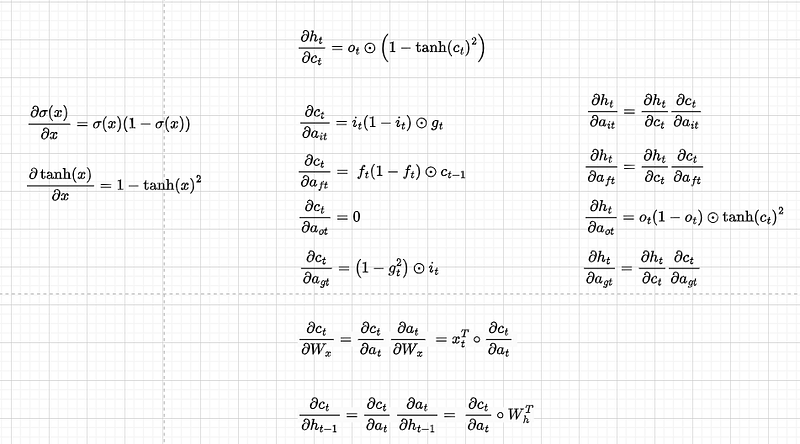
Note that for convenience, we have separated dct/dat and dht/dat, and wherever we have dht/dct dct/dat we write it directly as dht/dat. Also, because we will do back-propagation in the matrix form, we concatenate the derivatives of the gates in the following way:
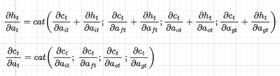
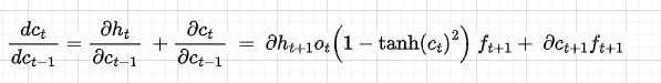
The sum in the dht/dat comes from the fact that we have two directions (see Figure 7) — one that goes into the previous cell and the other that goes into the hidden state. With the same logic of the gradient flow, the derivative of dct/dc(t-1) is as follows:
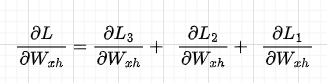
Now, let’s derive the total gradient with respect to Wx. This is given by the sum of the single losses with respect to Wx as described in part 1 of this series:
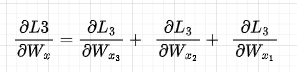
Focusing on individual loss, e.g., dL3/dWx, when we propagate from L3 to Wx, Wx appears in all the time-steps components thus, we will need to sum all these components to get the full gradient of L3 w.r.t. Wx. Slightly abusing mathematical notation, we are doing something like this (remember that Wx3 = Wx2 = Wx1):
The first component is going to be as below. Also, we replace dht/dct dct/dat with dht/dat so we then directly use that derivative
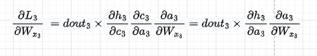
I will skip dL3/dWx2 for brevity and will jump directly into the third component. We have:
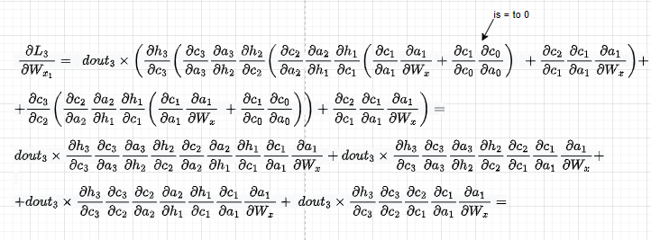
As previously, let’s replace wherever we have dht/dct dct/dat with dht/dat so we then directly use that derivative:
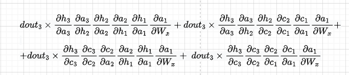
Summing them up, we get the derivative of dL3/dWx. To get the derivative of dWx w.r.t. the total loss, we will need to add to dL3/dWx, dL2/dWx, and dL1/dWx.
In code:
def lstm_forward(x, h0, Wx, Wh, b, next_c=None):
    h, cache = None, None

    cache = []
    N, T, _ = x.shape
    H = h0.shape[-1]
    h = np.zeros((N, T, H))
    if next_c is None:
        next_c = np.zeros((N, H))
    for t in range(x.shape[1]):
        xt = x[:, t , :]
        if t == 0:
            next_h, next_c, cache_s = lstm_step_forward(xt, h0, next_c, Wx, Wh, b)
            cache.append(cache_s)
        else:
            next_h, next_c, cache_s = lstm_step_forward(xt, next_h, next_c, Wx, Wh, b)
            cache.append(cache_s)

        h[:, t, :] = next_h

    return h, cache

def dc_da(h, prev_c, next_c_t, i, f, o, g):
    dgrad_c = np.zeros((h.shape[0], 4 * h.shape[1]))
    dgrad_h = np.zeros((h.shape[0], 4 * h.shape[1]))
    # assert dgrad.shape[1] % 4 == 0
    H = dgrad.shape[1] // 4

    # compute gradients wrt ai, af, ao and ag from two flows - next_h and next_c
    dnextc_dai = (i * (1-i)) * g
    dnextc_daf = (f * (1-f)) * prev_c
    dnextc_dao = 0
    dnextc_dag = (1 - g**2) * i

    dh_dc = o * (1 - next_c_t**2)

    dnexth_dai = dh_dc * dnextc_dai
    dnexth_daf = dh_dc * dnextc_daf
    dnexth_dao = (o * (1-o) * next_c_t)
    dnexth_dag = dh_dc * dnextc_dag

    # join them together in a matrix at this point to conveniently compute
    # downstream gradients
    dgrad_c[:, 0:H] = dnextc_dai
    dgrad_c[:, H:2*H] = dnextc_daf
    dgrad_c[:, 2*H:3*H] = dnextc_dao
    dgrad_c[:, 3*H:4*H] = dnextc_dag

    dgrad_h[:, 0:H] =  dnexth_dai
    dgrad_h[:, H:2*H] = dnexth_daf
    dgrad_h[:, 2*H:3*H] = dnexth_dao
    dgrad_h[:, 3*H:4*H] = dnexth_dag
    return dgrad_c, dgrad_h

np.random.seed(1)

N, D, T, H = 1, 3, 3, 1

x = np.random.randn(N, T, D)
h0 = np.random.randn(N, H)
Wx = np.random.randn(D, 4 * H)
Wh = np.random.randn(H, 4 * H)
b = np.random.randn(4 * H)

out, cache = lstm_forward(x, h0, Wx, Wh, b)

# let's define the dout instead of deriving them for simplicity
dout = np.random.randn(*out.shape)

# dL3/dWvx
dnext_c2 = np.zeros((h0.shape))
dnext_h2 = dout[:, -1, :]
(x2, next_h, prev_h, prev_c, Wx, Wh, next_h, next_c_t2, i2, f2, o2 ,g2) = cache[2]
dgrad_c2, dgrad_h2 = dc_da(h0, cache[2][3], cache[2][-5], cache[2][-4],  cache[2][-3], cache[2][-2], cache[2][-1])

dL3_dWx2 = x2.T @ (dgrad_h2 * dnext_h2 + dgrad_c2 * dnext_c2)
print(dL3_dWx2)

dnext_c1 = dnext_c2 * f2 + dnext_h2 * o2 * (1 - next_c_t2**2) * f2
dnext_h1 = (dnext_h2 * dgrad_h2 +  dnext_c2 * dgrad_c2) @ Wh.T

(x1, next_h, prev_h, prev_c, Wx, Wh, next_h, next_c_t1, i1, f1, o1 ,g1) = cache[1]
dgrad_c1, dgrad_h1 = dc_da(h0, cache[1][3], cache[1][-5], cache[1][-4],  cache[1][-3], cache[1][-2], cache[1][-1])

dL3_dWx1 = x1.T @ (dnext_c1 * dgrad_c1 + dnext_h1 * dgrad_h1)

print(dL3_dWx1)

dnext_c0 = dnext_c1 * f1 + dnext_h1 * o1 * (1 - next_c_t1**2) * f1
dnext_h0 = (dnext_h1 * dgrad_h1 + dnext_c1 * dgrad_c1) @ Wh.T

(x0, next_h, prev_h, prev_c, Wx, Wh, next_h, next_c_t0, i0, f0, o0 ,g0) = cache[0]
dgrad_c0, dgrad_h0 = dc_da(h0, cache[0][3], cache[0][-5], cache[0][-4],  cache[0][-3], cache[0][-2], cache[0][-1])

dL3_dWx0 = x0.T @ (dnext_c0 * dgrad_c0 + dnext_h0 * dgrad_h0)
print(dL3_dWx0)
Outputs:
[[-0.02349287  0.00135057 -0.11156069 -0.05284914]
 [ 0.01024921 -0.00058921  0.04867045  0.02305643]
 [-0.00429567  0.00024695 -0.02039889 -0.00966347]]
[[-9.83990139e-03  6.78775168e-05 -1.10660923e-03  4.20773125e-04]
 [ 7.93641636e-03 -5.47469140e-05  8.92540613e-04 -3.39376441e-04]
 [-2.11067811e-02  1.45598602e-04 -2.37369846e-03  9.02566589e-04]]
[[-1.95768961e-05  0.00000000e+00  2.77411349e-05 -9.76467796e-03]
 [ 7.37299593e-06  0.00000000e+00 -1.04477887e-05  3.67754574e-03]
 [ 6.36561888e-06  0.00000000e+00 -9.02030083e-06  3.17508036e-03]]
losses_dWx = {i : {x_comp : 0 for x_comp in range(i)} for i in range(T)}
dWx = np.zeros((D, 4 * H))
dWh = np.zeros((H, 4 * H))
db = np.zeros((4 * H, ))
for idx in range(T-1, -1, -1):
print(f"Loss {idx + 1}")
dnext_c = np.zeros((h0.shape))
dnext_h = dout[:, idx, :]
for j in range(idx, -1, -1):
(x, next_h, prev_h, prev_c, Wx, Wh, next_h, next_c_t, i, f, o ,g) = cache[j]
dgrad_c, dgrad_h = dc_da(h0, prev_c, next_c_t, i, f, o, g)
dgrad = dnext_c * dgrad_c + dnext_h * dgrad_h
losses_dWx[idx][j] = x.T @ dgrad
dnext_c = dnext_c * f + dnext_h * o * (1 - next_c_t**2) * f
dnext_h = (dnext_h * dgrad_h + dnext_c * dgrad_c) @ Wh.T
dnext_h = dgrad @ Wh.T
# accumulate gradient of dWx and other params for each loss
dWx += x.T @ dgrad
dWh += prev_h.T @ dgrad
db += dgrad.sum(0)
print(f"component {j} - ", np.linalg.norm(losses_dWx[idx][j]))Vanishing gradient in LSTM
As in part 1 for RNN, let’s see the gradients for the Loss L3 for each component:
Loss 3
component 0 - 0.010906688399113558
component 1 - 0.02478099846737857
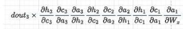
component 2 - 0.13901933055672275From the above, we can see that X3 (component 2), which is the closest to L3 still has the largest update, while X1 and X2 contribute less to Wx1 update. For RNN this difference is much larger, however. Indeed, the gradient that passes through the hidden state will suffer from the vanishing gradient for the same reason as RNN — Wh terms (dat/dh(t-1)) still appear in the back-propagation, for example here in dL3/dWx1 (Figure 15):
However, the gradient that flows through the cell that is still a function of the input and of the hidden state does not have Wh terms but sigmoid terms instead (see the formula for forget gate ft in Figure 3):
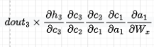
Recall that dct/dc(t-1) = ft. Thus, if forget gate is high, i.e., close to 1, then the vanishing gradient happens at a much slower rate than in vanilla RNN, but it will still happen unless all the forget gates are exactly 1, which does not happen in practice.
Conclusions
The main point of this article was to understand, by deriving back-propagation, that LSTM still suffers from the vanishing gradient in practice, however, at a much lower rate than vanilla RNN thanks to the cell state, which makes the gradient decay at forget gate rate rather than Wx rate. If you find any errors, please let me know in the comments.


