A Deep Dive into the Code of the BERT Model

Breaking down the HuggingFace BERT Implementation

There are already many tutorials out there on how to create a simplified Bert model from scratch and how it works. In this article we are going to do something slightly different — we go through the actual Hugging face implementation of BERT breaking down all its components.

Introduction

Transformer models revolutionised the NLP space in the last few years. BERT (Bidirectional Encoder Representations from Transformers) is one of the most successful Transformers — it outperformed on a variety of tasks previous SOTA models like LSTM both in performance thanks to a better context understanding through attention mechanisms and training time because differently from LSTM’s recursive structure, BERT is parallelizable.

Now without waiting any longer, let’s dive into the code and see how it works. First we load the Bert model and output the BertModel architecture:

We analyse separately the 3 parts: Embeddings, Encoder with 12 repeating Bert layers and Pooler. Eventually we will add a Classification Layer.

BertEmbeddings : Starting from raw text, first thing to do is to split our sentences into tokens that we can then pass to BertEmbeddings. We use BertTokenizer that is based on WordPiece — subword tokenization trainable algorithm which helps to balance the vocabulary size and out of vocabulary words. Unseen words are split into subwords, which are derived during the training stage of the tokenizer (more details on this here). Let’s now import few sentences from 20newsgroups dataset and tokenize them

from sklearn.datasets import fetch_20newsgroups
newsgroups_train = fetch_20newsgroups(subset='train')

inputs_tests = tokenizer(newsgroups_train['data'][:3], truncation=True, padding=True, max_length=max_length, return_tensors='pt')

Once the sentences are split into tokens we assign each token a representative numerical vector that represents that token in a n dimensional space. Each dimension holds some information of that word, so if we assume features are Wealth, Gender, Cuddly the model, after training the embedding layer, will represent for example the word king with the following 3 dimensional vector: (0.98, 1, 0.01) and cat with (0.02, 0.5, 1). We can then can use those vectors to compute the similarity between words (using cosine distance) and do many other things.

NB: in reality we cannot derive what those features names really are, but it’s helpful to think of them that way to have a clearer picture.

So word_embeddings is a matrix of shape in this case (30522, 768) where the first dimension is the vocabulary dimension, while the second is embedding dimension, i.e. the number of features with which we represent a word. For base-bert it’s 768 and it increases for bigger models. In general the higher the embedding dimension the better we can represent certain words — this is true to a degree, at some point increasing the dimension will not increase the accuracy of the model by much while computational complexity does.

model.embeddings.word_embeddings.weight.shape
output: torch.Size([30522, 768])

position_embeddings is needed because, differently from LSTM model for example which processes tokens sequentially and hence has the sequential information of each token by construction, Bert model processes tokens in parallel and to incorporate positional information of each token we need to add this information from position_embeddings matrix. The shape of it is (256, 768) where the former represents the max sentence length whilst the latter is the features dimension as for word embeddings — so depending on the position of each token we retrieve the associated vector. In this case we can see that this matrix is learnt, but there are other implementations where it’s built using sines and cosines.

model.embeddings.position_embeddings.weight.shapeoutput: torch.Size([256, 768])

token_type_embeddings is “redundant” here and comes from the Bert training task where the semantic similarity between two sentences is assessed — this embedding is needed to distinguish between the first and the second sentence. We do not need it as we have only one input sentence for classification task.

Once we extract the words embeddings, positional embeddings and type embeddings for each word in the sentence we just sum them up to get the full sentence embedding. So for the first sentence it will be:

For our mini-batch of 3 sentences, we can get them in the following way:

Next we have a LayerNorm step which helps the model to train faster and generalize better. We standardize each token’s embedding by token’s mean embedding and standard deviation so that it has zero mean and unit variance. We then apply a trained weight and bias vectors so it can be shifted to have a different mean and variance so the model during training can adapt automatically. Because we compute mean and standard deviation across different examples independently from the others, it is different from Batch normalization where the normalization is across the batch dimension and thus depends on other examples in the batch.

Let’s finally apply Dropout, where we replace with zero some of the values with certain dropout probability. Dropout helps to reduce overfitting as we randomly block signals from certain neurons so the network needs to find other paths to reduce the loss function, and thus it learns how to generalise better instead of relying on certain paths. We can also see dropout as a kind of models ensembling technique as during training at each step we randomly deactivate certain neurons ending up with “different” networks which we eventually ensemble during the evaluation time.

NB: because we set model to evaluation mode we will ignore all the dropout layers, they are only used during training. We still include it for completeness.

norm_embs_dropout = model.embeddings.dropout(norm_embs)

We can check that we obtain the same results as from the model:

embs_model = model.embeddings(inputs_tests[‘input_ids’], inputs_tests[‘token_type_ids’])
torch.allclose(embs_model, norm_embs, atol=1e-06) # True

Encoder

The encoder is where most of the magic happens. There are 12 BertLayers and the output of the previous is fed into the next. This is where attention is used to create different representations of the original embeddings that are context-dependent. Within the BertLayer we first try to understand BertAttention — after deriving the embeddings of each word, Bert uses 3 matrices — Key, Query and Value, to compute attention scores and derive the new values for words embedding based on other words in the sentences; this way Bert is context aware, embedding of each word instead of being fixed and context independent is derived based on other words in the sentence and the importance of other words when deriving new embedding for a certain word is represented by the attention score. To derive the query and key vector for each word we need to multiply its embedding by a trained matrix (which are separate for Queries and Keys). For example, to derive the query vector for the first word of the first sentence :

We can notice that of the entire query and key matrices we only select the first 64 (=att_head_size) columns (the reason will be clarified shortly) — this is the new embedding dimension of the words after the transformation and it’s smaller than the original embedding dimension 768. It is done to reduce the computational burden but having actually a longer embedding might lead to a better performance. Indeed it’s a trade off between reduction in complexity and increase in performance. Now we can derive the Query and Key matrices for the entire sentence:

To compute attention score we multiply Query matrix by Key matrix and standardize it by the square root of the new embedding dimension (=64=att_head_size). We also add to it a modified attention mask. Initial attention mask (inputs[‘attention_mask’][0]) is a tensor of 1s and 0s where 1 means that there is a token in that position and 0 that it’s a padded token. If we subtract from 1 the attention mask and multiply it by a high negative number, when we apply SoftMax we effectively send to zero those negative values and then derive probabilities based on other values. Let’s see the example below:

If we have a sentence of 3 tokens + 2 paddings, we get the following attention mask for it: [0,0,0, -10000, -10000] Let’s apply the SoftMax function:

Let’s check if the attention scores we derived are the same we get from the model. We can get the attention scores from the model with the following code:

as we defined output_attentions=True, output_hidden_states=True, return_dict=True we will get last_hidden_state, pooler_output, hidden_states for each layer and attentions for each layer

out_view = model(**inputs_tests)

out_view contains:

• last_hidden_state (batch_size, sequence_length, hidden_size) : last hidden state which is outputted from the last BertLayer
• pooler_output (batch_size, hidden_size) : output of the Pooler layer
• hidden_states (batch_size, sequence_length, hidden_size): hidden-states of the model at the output of each BertLayer plus the initial embedding
• attentions (batch_size, num_heads, sequence_length, sequence_length): one for each BertLayer. Attentions weights after the attention SoftMax

torch.allclose(attention_scores, out_view[-1][0][‘attn’][0, 0, :, :], atol=1e-06)) # True

print(attention_scores[0, :])
tensor([1.0590e-04, 2.1429e-03, .... , 4.8982e-05], grad_fn=<SliceBackward>)

The first row of the attention score matrix says that, to create the new embedding for the first token, we need to attend to the first token (to itself) with weight = 1.0590e-04, second token with weight = 2.1429e-03 and so on. In other words, if we multiply by those score the vectors embeddings of the other tokens we derive the new representation for the first token, but, instead of actually using the embeddings we will use the Value matrix which is computed below.

Value matrix is derived in the same way as Query and Key matrices:

We then multiply these Values by the attention scores to get the new context-aware words representations

new_embed_1 = (attention_scores @ V_first_head)

Now you might be wondering, why we are selecting the first 64 (=att_head_size) elements from the tensors. Well, what we have computed above is one head of the Bert attention layer, but actually there are 12 of them. Each of these attention heads creates different representation of words (new_embed_1 matrix) where for example given the following sentence “I like to eat pizza in the Italian restaurants”, in the first head the word “pizza” might pay attention mostly to the previous word, the word itself and the following word and remaining words will have close to zero attention. In the next head, it might pay attention to all verbs (like and eat) and would capture this way different relationships from the first head.

Now, instead of deriving each head separately we can derive them together in the matrix form:

The attention from the first example and the first head is the same we derived before :

example = 0
head = 0
torch.allclose(attention_scores, attention_probs[example][head]) # True

We now concatenate the results from the 12 heads and pass them through a bunch of linear layers, Normalization Layers and dropouts that we have already seen in the embedding part to get the result of the encoder for the first layer.

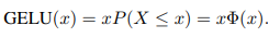
output_dense we are simply passing our concatenated attention results through a linear layer. We then need to normalize, but we can see that instead of normalizing the output_dense immediately, we first sum it to our initial embeddings — this is called Residual connection. When we increase the depth of a neural network, i.e., stacking more and more layers we bump into the problem of vanishing/exploding gradients, when in case of vanishing gradients the model is not able to learn anymore as the propagated gradients are close to zero and initial layers stop changing weights and improve. Opposite problem with exploding gradients when the weights cannot stabilize because of extreme updates which eventually explode (go to infinity). Now, proper initialisation of weights and normalization helps to address this problem but what has been observed is even if the network becomes more stable, the performance decreases as the optimization is harder. Adding these residual connections helps to improve performance and the network becomes easier to optimize even if we keep increasing depth. Residual connection is also used in out_layernorm which is actually the output of the first BertLayer. Last thing to notice is when we compute interm_dense , after passing the output from AttentionLayer through a linear layer, a non linear GeLU activation function is applied. GeLU is represented as:

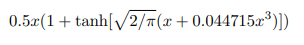
But it’s approximated with the following formula for faster calculations:

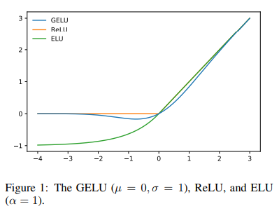
Looking at the graph we can see that if ReLU, that is given by the formula max(input, 0), is monotonic, convex and linear in the positive domain, GeLU is non-monotonic, non-convex and non-linear in the positive domain and thus can approximate more easily complicated functions.

We have now successfully reproduced an entire BertLayer. The output of this layer (same shape as the initial embedding) goes into the next BertLayer and so on. There are overall 12 BertLayers. So putting all of these together we can get the final results from the encoder for all 3 the examples:

Note how out_layernorm — the output of each layer is fed into the next layer.

And we can see that this is the same result as in out_view

torch.allclose(out_view[-2][-1], out_layernorm, atol=1e-05) # True

Pooler

Now we can take the first token output of the last BertLayer, which is [CLS], pass it through a Linear layer and apply a Tanh activation function to get the pooled output. The reason to use the first token for classification comes from how the model was trained as the authors of Bert state:

The first token of every sequence is always a special classification token ([CLS]). The final hidden state corresponding to this token is used as the aggregate sequence representation for classification tasks.

out_pooler = torch.nn.functional.tanh(out_layernorm[:, 0] @ model.pooler.dense.weight.T + model.pooler.dense.bias)

Classifier

Finally we create a simple class which will be a simple Linear layer, but you can add a dropout to it and other things. We assume a binary classification problem here (output_dim=2), but it can be of any dimension.

from torch import nn
class Classifier(nn.Module):
    
    def __init__(self, output_dim=2):
        super(Classifier, self).__init__()
        self.classifier = nn.Linear(model.config.hidden_size, output_dim, bias=True)
    
    def forward(self, x):
        return self.classifier(x)

classif = Classifier()
classif(out_pooler)

tensor([[-0.2918, -0.5782],
        [ 0.2494, -0.1955],
        [ 0.1814,  0.3971]], grad_fn=<AddmmBackward>)

Conclusions

Now you should understand every single building block of Bert, thus the next step is the actual application! In the next article we will show Bert in action, and how to monitor the training with TensorBoard which helps to spot very early if something is wrong in the training process.

References

https://arxiv.org/pdf/1606.08415v3.pdf https://arxiv.org/pdf/1810.04805.pdf https://jalammar.github.io/illustrated-transformer/ https://github.com/huggingface/transformers/