
A Complete Guide to twitter Sentiment Analysis — Part II
A follow-along tutorial to guide you through the in-depth twitter sentiment analysis using Python
Sentiment Analysis is the method to measure attitude and emotions of a speaker/writer based on computational treatment of text data. Sentiment analysis could be very useful for businesses to understand the social sentiment of their brand, product or service while monitoring online conversations.
This article is part 2 of the 2-part series that guides you through the complete process of sentiment analysis of Twitter data using Python.
In the last part we saw how to scrape the tweets using a library called Tweepy in Python. We scraped tweets on the topic ‘covid’. We also did some hashtag analysis, basic text cleaning and calculated average length of texts and average word counts of the tweets. Part I of this tutorial can be found here. In this tutorial let’s learn to perform sentiment analysis of the tweets.

1. Sentiment Analysis
Sentiment analysis could be performed in Python using 2 methods — i) Calculating polarity and subjectivity using the library Textblob. ii) Using senimentIntensityAnalyzer from the library vader. A brief comparison of both the libraries can be found here.
I decided to use the Vader library because it works well with the social media data. The SentimentIntensityAnalyzer function relies on a dictionary that maps lexical features to emotion intensities known as sentiment scores. The sentiment score of a text can be obtained by summing up the intensity of each word in the text.
This function analyzes the text and returns the score in the form of a dictionary with the following components :negative, neutral, positive and compound. Based on the scores assigned to each component, we can define the overall sentiment of the text to be positive, negative or neutral. This is done in the following code:
import nltk
nltk.download('vader_lexicon')
from nltk.sentiment.vader import SentimentIntensityAnalyzer
for index, row in tweets_df['Text'].iteritems():
score = SentimentIntensityAnalyzer().polarity_scores(row)
if score['neg'] > score['pos']:
tweets_df.loc[index, "Sentiment"] = "negative"
elif score['pos'] > score['neg']:
tweets_df.loc[index, "Sentiment"] = "positive"
else:
tweets_df.loc[index, "Sentiment"] = "neutral"
tweets_df.loc[index, 'neg'] = score['neg']
tweets_df.loc[index, 'neu'] = score['neu']
tweets_df.loc[index, 'pos'] = score['pos']
tweets_df.loc[index, 'compound'] = score['compound']
tweets_df.head(10)2. Visualize the sentiment Counts
Once the sentiments are identified, we can create 3 lists for different sentiments. We can then calculate the overall percentage of each sentiment in the dataset.
#create new data frames for all sentiments
tweet_neg = tweets_df[tweets_df["Sentiment"] == "negative"]
tweet_neu = tweets_df[tweets_df["Sentiment"] == "neutral"]
tweet_pos = tweets_df[tweets_df["Sentiment"] == "positive"]#function for calculating the percentage of all the sentiments
def calc_percentage(x,y):
return x/y * 100pos_per = calc_percentage(len(tweet_pos), len(tweets_df))
neg_per = calc_percentage(len(tweet_neg), len(tweets_df))
neu_per = calc_percentage(len(tweet_neu), len(tweets_df))print("positive: {} {}%".format(len(tweet_pos), format(pos_per, '.1f')))
print("negative: {} {}%".format(len(tweet_neg), format(neg_per, '.1f')))
print("neutral: {} {}%".format(len(tweet_neu), format(neu_per, '.1f')))format(calc_percentage(len(tweet_neu), len(tweets_df)), '.1f')))The output obtained from the code above:
positive: 1788 35.8%
negative: 1795 35.9%
neutral: 1417 28.3%
Example of some of the tweets classified as positive:
2    The economy is roaring back. Kids are returning to school. Things are looking up. Get vaccinated and let's keep it going.
3    Help slow the spread   of  and identify at risk cases sooner   by selfreporting your symptoms daily, even if you feel well . Download the   app
7    Cholesterol drug cuts coronavirus infection by 70, researchers find
10    Coronavirus weekly   needtoknow Long COVID, delta variant, ivermectin drug  more
11    Meet Pokaa the Golden Labrador, the sniffer dog in France with 100  success rate in detecting coronavirus in under 10 minutes, 48 hours quicker than a PCR lab test
Sample of some of the tweets classified as negative:
1    150 children dying EVERY WEEK from Covid 19 in Indonesia  Devastating  Children are not safe from
6    It seems we've entered a point where  ended and now they are just making shit up about the Common Cold or whatever to keep us locked down and sheltered from our freedoms.
9    Ive cared for children whose entire families have been devastated by sometimes the childhad no parent at their bedside bc the parents were critically ill
13    has been extraordinarily hard on   in particular small businesses. Read to learn more about the local impact and what future needs are
14   Was there anyone on this planet that believed the Delta Variant sidestepped Japan Did anyone on this planet think they were safe from Delta coronavirus if the were in Japan  The Delta variant has circumnavigated the globe, pretty sure CVdelta is everywhere
Next, we can plot a bar graph to understand the distribution of sentiments amongst the tweets.
#create a bar graph by sentiment
import matplotlib.pyplot as plt
labels = tweets_df.groupby('Sentiment').count().index.values
values = tweets_df.groupby('Sentiment').size().values
plt.bar(labels, values)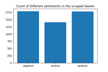
A pie chart would also be a good representation to display various sentiments amongst the data. This is done as follows:
labels = ['Positive ['+format(pos_per, '.1f')+'%]', 'Neutral ['+format(neu_per,'.1f')+'%]', 'Negative ['+format(neg_per,'.1f')+'%]']
sizes = [len(tweet_pos), len(tweet_neu), len(tweet_neg)]
colors = ['green', 'blue', 'red']
patches, texts = plt.pie(sizes, labels = labels, colors = colors,shadow = True, startangle = 90)
plt.legend(labels)
plt.title("Sentiment Analysis of Tweets")
plt.axis('equal')
plt.show()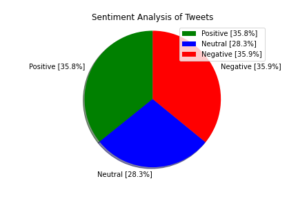
3. Creating Word clouds
In order to understand which words have been used most in the tweets, we can create a word cloud. WordCloud function from the library wordcloud has been used for the same. I defined a function for creating a word-cloud and the same function has been called to create clouds for positive tweets as well as negative tweets.
from wordcloud import WordCloud, STOPWORDS
#function to create word cloud
def create_wordcloud(text):
    stopwords = set(STOPWORDS)
    wc = WordCloud(background_color = "white", max_words = 3000, stopwords = stopwords, repeat = True)
    wc.generate(str(text))
    plt.imshow(wc, interpolation='bilinear')
    plt.axis("off")
    plt.show()
#word cloud for positive sentiments
create_wordcloud(tweet_pos["Cleaned_Text"].values)#wordcloud for negative sentimenst
create_wordcloud(tweet_neg["Cleaned_Text"].values)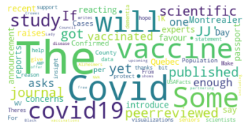
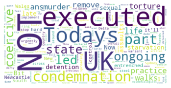
We can see from the word clouds of positive and negative tweets that most popular words for positive tweets are Covid, vaccine, scientific, published, reports etc. Some common words for negative tweets are condemnation, executed, murder, torture etc.
WordCloud function plots the popular words in the corpus by their frequencies. More is the frequency of a word in the corpus, bigger is the size of the word in the cloud. We can change this behavior by passing a dictionary and generating the cloud using pre-calculated frequencies. For this, we use the function ‘generate_from_frequencies’ in the above code in place of ‘generate’.
We can also be creative with the shape of word clouds. They don’t have to be boring rectangles. We can create clouds in many different shapes and experiment with the color schemes and backgrounds too.
4. Find the Most popular words in the tweets and their frequencies
To find popular words in the text data, we have to perform vectorization. For this, we first start with tokenization, where every word is converted to a single entity called token. Next, we remove stop words. Stop words are the common words used in the English language like ‘is’, ‘on’, ‘the’ etc. Next, we perform lemmatization. Lemmatization is the process of grouping words together so that they can be analyzed as single item. For example, words like joined, joint, joining are all grouped as a single word- join.
#Apply tokenization
def tokenization(text):
    text = re.split('\W+', text)
return texttweets_df['tokenized'] = tweets_df['Cleaned_Text'].apply(lambda x: tokenization(x.lower()))#Removing Stop words
stopword = nltk.corpus.stopwords.words('english')
def remove_stopwords(text):
text = [word for word in text if word not in stopword]
return texttweets_df['nonstop'] = tweets_df['tokenized'].apply(lambda x:remove_stopwords(x))#Stemmer
ps = nltk.PorterStemmer()
def stemming(text):
text = [ps.stem(word) for word in text]
return texttweets_df['stemmed'] = tweets_df['nonstop'].apply(lambda x: stemming(x))#join all the words to make a final text field
tweets_df['final'] = tweets_df['stemmed'].apply(lambda x: ' '.join(x))
tweets_df.head()Next we perform vectorization of texts, which is a methodology to map words in the vocabulary to a corresponding vector of real numbers. Every tweet in the dataset is treated as a document and every word in the tweets is treated as a feature. The texts are then converted to a document feature matrix. If a word is present in the tweet, it is represented by the number of times it occurs in that tweet, 0 otherwise.
#applying count vectorizer
from sklearn.feature_extraction.text import CountVectorizer
countVectorizer = CountVectorizer()
countVector = countVectorizer.fit_transform(tweets_df['final'])
print('{} Number of tweets have {} words'.format(countVector.shape[0], countVector.shape[1]))
5000 Number of tweets have 8505 wordscount_vect_df = pd.DataFrame(countVector.toarray(), columns = countVectorizer.get_feature_names())
count_vect_dfWith the help of count vector thus created, we can now find the most popular words in the tweets. Top 10 words from the dataset can be displayed as below
#most frequently used words in the tweets
counts = pd.DataFrame(count_vect_df.sum())
count_df = counts.sort_values(0, ascending = False).head(10)
count_df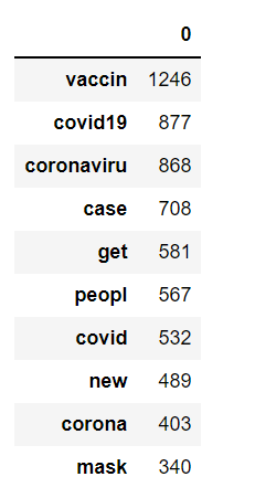
We can also create a bar graph of the frequencies of the most popular words to understand their distribution.
#create a bar graph of most frequently used words
ind = count_df.index
val = [item for sublist in count_df.values for item in sublist]plt.bar(ind, val)
plt.xticks(rotation = 90)
plt.title('Top 20 Most frequently used words in the tweets')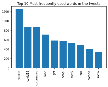
We can do similar analysis on the data frames of positive and negative tweets to understand the frequency distribution of all the popular words in them.
Conclusion
This concludes the twitter sentiment analysis — part II. There are many more analysis techniques that you can apply on the twitter data like topic modelling(divide the tweets into different topics. An example of topic modelling in R can be found here). Other techniques are geospatial analysis, text similarity and knowledge graphs. The possibilities are endless.
If this tutorial was worth your time, please feel free to clap and follow. Say Hi on linkedin if you like.