Scraping and analyzing tweets in R

Learn to scrape data from the twitter and perform topic modelling in R

January 2021 was an important month in the US political history for many reasons. First, because Joe Biden was declared the winner of US presidential election 2020. Second, because hundreds of Trump supporters stormed the Capitol building to show their support for Donald Trump. Third, because Covid vaccination rollout began in January. During all these events, lots of tweets were made by global political leaders about the events happening around.

In this analysis project, let’s try to scrape the tweets made by Joe Biden from the twitter during the last month and do topic modelling by dividing them into different topics.

Step 1: Get API access from Twitter

For scraping data from the twitter, you first need to create a twitter developer account here. Once this is done, you get the authorization code for accessing the tweets. Detailed instructions for the same could be found here.

my_authorization <- rtweet::create_token(app = "your app name",
 consumer_key = "your consumer key",
 consumer_secret = "your consumer secret", access_token="your access token", access_secret = "Your access secret")

Step 2 : Scrape the tweets

Using the authorization code generated above, we scrape the tweets from Jo Biden’s twitter account and save in a .csv file.

biden_tweets <- rtweet::get_timeline(c("joebiden"), n = 3000, parse=T, token=my_authorization)
rtweet::write_as_csv(biden_tweets, "biden_tweets.csv", prepend_ids = TRUE, na = "", fileEncoding = "UTF-8")

We can check the .csv file to see that there are 3000 rows(as specified by us) and 90 different columns with details like date, the tweet is created on, text of the tweet, hashtags, number of times retweeted etc.

Step 3 : Analyse the tweets

The csv file is then read using the readtext function from the readtext library. Readtext library makes it easier to import the text files in various formats, and returns a data frame, that is easy to manipulate.

bidenTexts <- readtext::readtext("biden_tweets.csv", text_field = "text")
dim(bidenTexts)

Let us now retrieve 5 top tweets that have been most popular and have been retweeted the maximum times.

head(bidenTexts[order(-bidenTexts$retweet_count), 'text' ],5)

We get the following answer:-

[1]“America, I’m honored that you have chosen me to lead our great country.\n\nThe work ahead of us will be hard, but I promise you this: I will be a President for all Americans — whether you voted for me or not.\n\nI will keep the faith that you have placed in me. https://t.co/moA9qhmjn8" [2] “We did it, @JoeBiden. https://t.co/oCgeylsjB4" [3] “It’s a new day in America.” [4] “My message to my fellow Americans and friends around the world following this week’s attack on the Capitol. https://t.co/blOy35LWJ5” [5] “I can’t believe I have to say this, but please don’t drink bleach.”

Similarly, we can analyze the data frame to retrieve the tweets that have been marked as favourite the maximum number of times.

head(bidenTexts[order(-bidenTexts$favorite_count), 'text'], 5)

[1] “It’s a new day in America.” [2] “America, I’m honored that you have chosen me to lead our great country.\n\nThe work ahead of us will be hard, but I promise you this: I will be a President for all Americans — whether you voted for me or not.\n\nI will keep the faith that you have placed in me. https://t.co/moA9qhmjn8" [3] “Keep the faith, guys. We’re gonna win this.” [4] “Donald Trump is the worst president we’ve ever had.” [5] “America is back.”

Step 4: Find the most frequently used words and topics

We start by creating a corpus for the tweets. The corpus function converts every tweet to a documents with features like number of tokens in the document, type, user id, text width etc. We can get the list of all the features using the summary command.

#create a corpus
bidenCorpus<-quanteda::corpus(bidenTexts)
summary(bidenCorpus)
dfmbiden <- dfm(bidenCorpus, remove = c(stopwords("english")),
                remove_punct = TRUE, remove_numbers = TRUE,    remove_symbol = TRUE,tolower=T)

We then use the dfm function to convert the corpus into document feature matrix, which represents the counts of features by documents. In the document feature matrix, the corpus is converted into a sparse matrix with as many rows as there are documents in the corpus and as many features as there are words in the corpus. If a word is present in a document, it is represented by the number of times it occurs in the document, 0 otherwise. While doing this, we have also removed the stop words like ‘if’, ‘an’ etc, and removed symbols, numbers, and punctuations.

To see which words have been used mostly by Biden in his tweets, we can draw a word cloud using textplot_wordcloud function from the library quanteda.

set.seed(111)
quanteda::textplot_wordcloud(dfmbiden, max_words = 150, color = RColorBrewer::brewer.pal(8, "Dark2"))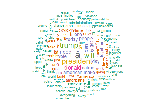

Let us now try to do the topic modelling, which divides the tweets into different topics. For this, we first define a dictionary with example words for each topic. We have defined 10 topics for this analysis. Tweets that do not fall into any of these topics would be segmented as ’other’.

dict <- dictionary(list(capitol_attack = c("attack", "responsibility", "capitol", "shame", "storming"),
        cabinet = c("cabinet", "minister", "advisory"),
        education = c("school", "education"),
        employment = c("job", "right", "wage","employment"),
        winning = c("victory", "win", "thank", "america","great", "back", "proud"),
        economy = c("poverty","crisis", "society", "job*", "rent", "relief" ),
        war = c("war", "soldier*", "nuclear"),
        crime = c("crime*", "murder", "killer", "violence"),
        corona = c("covid-19", "corona", "pandemic", "virus", "mask", "vaccine"),
        trump = c("trump", "donald","president", "law" )))

We now use textmodel_seededlda() from the library seededlda to implement semi-supervised Latent Dirichlet allocation (seeded-LDA). Without going into the details of the algorithm, it is enough to know that this algorithm divides texts into pre-defined topics. We do this by fitting seeded_lda model to the dfm defined above. We can then check the top words for every topic.

slda <- textmodel_seededlda(dfmbiden_tfidf, dict, residual = TRUE)
topwords_biden <- as.data.frame(seededlda::terms(slda, 20))

Now, we store the topics thus identified into a “topic” column of our data frame. After that, we tabulate the frequencies of each topic in our corpus and create a proportion table for the same.

bidenTweets$topic <- seededlda::topics(slda)

#tabulate frequencies of each topic in your corpus:
topics_table <-ftable(bidenTweets$topic)
topicsprop_table <- as.data.frame(prop.table(topics_table))

Lastly, all that we need to do is plot the topics according to their frequencies in the proportion table.

ggplot(data=topicsprop_table, aes(x=Var1, y=Freq)) + 
  geom_bar(stat = "identity") +
  labs (x= "Topics", y = "Topic %")+
  labs(title = "Topic proportions - Biden") +
  theme(axis.text.x = element_text(face="bold", 
                                   size=10, angle=45,hjust = 1))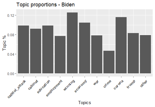

We can see from the bar graph above that out of the 3000 tweets made by Joe Biden in January, maximum(13%) were about his winning the election, followed by Covid-19(11%) and economy(9%).

In this article, we learnt to scrape tweets from the twitter app and analysed them by the number of times they are retweeted or made favourite. We also learnt to plot a word cloud and do topic modelling. Detailed code for this article can be found on this link.

If you like the article please don’t forget to clap and follow.