A Beginner’s Guide to Similarity Search & Vector Indexing (Part Three)

Part 1, Part 2, and Part 3 of this series.

In the previous articles of this series, we explored the nuances of similarity search alongside three distinct indexing techniques: Flat, IVF, and HNSW, which can be revisited in our earlier discussions (article 1 and article 2). In this article we will explore additional Approximate Nearest Neighbor (ANN) methods pertinent to similarity search and indexing, specifically focusing on ANNOY, LSH, and Product Quantization methods. These approaches offer varied benefits in terms of search efficiency and precision, catering to diverse needs within the realm of data retrieval.

ANNOY (Approximate Nearest Neighbors Oh Yeah)

ANNOY is a similarity search algorithm designed for memory-efficient and fast retrieval of nearest neighbors in high-dimensional spaces. ANNOY is particularly well-suited for applications where fast query times and low memory footprint are required, even on very large datasets. Similar to other ANN techniques, ANNOY operates in two phases: building the a or forest structure, and then identifying the indexes of the vectors that are closest to the given query vector.

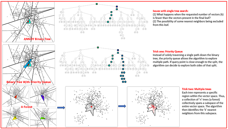
Constructing Tree/Forest Using ANNOY Algorithm: The ANNOY algorithm constructs a tree (or multiple trees for a forest) by recursively splitting the dataset with hyperplanes. It selects two random points to define each hyperplane and partitions the space into two, placing each point on the side of the hyperplane it’s closest to. This process repeats until each leaf node has a maximum of K points. For a forest, multiple trees are created with different random splits, enhancing the robustness of the search.

Finding Similar Vectors Using ANNOY Algorithm: The ANNOY algorithm finds similar vectors by traversing the trees in the forest, using hyperplanes at each node to guide the search towards the area of the tree where the nearest neighbors are likely to be. It employs a priority queue to efficiently explore tree branches, and by searching across multiple trees, it increases the probability of finding the true nearest neighbors. The final step involves calculating exact distances to a shortlist of close vectors to determine the most similar ones.

Priority Queue in ANNOY: In the ANNOY algorithm, a priority queue is employed as a strategic trick to enhance the search for similar vectors. Instead of solely traversing a single path down the binary tree, the priority queue allows the algorithm to explore multiple paths. Specifically, the priority queue is used to explore nodes sorted by the maximum distance into the “wrong” side of a split. This means that if a query point is “close enough” to a split, the algorithm can decide to explore both sides of that split. The threshold for determining “closeness” can be configured, and the priority queue aids in searching with increasingly larger thresholds, starting from zero. By utilizing a priority queue in this manner, ANNOY can more effectively and efficiently navigate the tree to find the most similar vectors to a given query point.

Forest Method for Efficient Nearest Neighbor Search in ANNOY: The forest method in ANNOY involves constructing multiple binary trees, collectively referred to as a “forest.” Each tree in this forest is constructed using a random set of splits. The idea behind building multiple trees is to increase the chances of finding favorable splits that can guide the search towards the true nearest neighbors. When querying for similar vectors, ANNOY doesn’t search just one tree but traverses all the trees in the forest simultaneously. This is achieved using a single priority queue, which helps in efficiently navigating through the trees. An added advantage of this method is that the search focuses more on the trees that are most relevant or “best” for each query, specifically those trees where the splits are furthest away from the query point. As every tree contains all the points, searching multiple trees means some points will be found in several trees. By looking at the union of the leaf nodes from all the trees, ANNOY can obtain a comprehensive neighborhood of potential nearest neighbors. This forest method significantly enhances the accuracy and efficiency of the nearest neighbor search in high-dimensional spaces.

The following image illustrates the functioning of the binary tree, the role of the priority queue, and the use of multiple trees in the ANNOY algorithm.

Taking from https://erikbern.com/2015/10/01/nearest-neighbors-and-vector-models-part-2-how-to-search-in-high-dimensional-spaces.html

Implementation of ANNOY: If you’re interested in giving this implementation a try, I encourage you to check out the previous article (part 1 & part 2) where we’ve explored other methods and data source. Like other ANN methods, it is also two step process: constructing index and querying neighbors. This algorimth is implemented in annoy library and most of its parameters are discribed in this Github Repository. The following piece of code shows how we can create index and make a similarity search using annoy library.

!pip install annoy
from annoy import AnnoyIndex
import pandas as pd
import faiss
df=pd.read_csv('https://raw.githubusercontent.com/DhunganaKB/customchat/main/VectorIndexSearch/TextClassification_Indexing.csv')
df = df.reset_index(drop=True)

## Creating embedding vectors
from sentence_transformers import SentenceTransformer
model = SentenceTransformer('bert-base-nli-mean-tokens')
sentences = list(df['Sentence'])
sentence_embeddings = model.encode(sentences)
embedding_dimension = sentence_embeddings.shape[1]
print(embedding_dimension)

# here we are choosing default angular (angle between vectors) option
index = AnnoyIndex(embedding_dimension)
# we can choose other similarity metric such as
t = AnnoyIndex(embedding_dimension, 'euclidean')  # For Euclidean distance

# adding items (vectors) to index

for i, vector in enumerate(sentence_embeddings):
    index.add_item(i, vector)

# building the index with 10 tree
index.build(n_trees=10)

# want to choose three nearest neighbors 
k=3
# creating query vector from plain text
# please check part 1 and part 2 of this serie
xq=model.encode(['I would like to know about Nobel Prize from 2020'])

I = index.get_nns_by_vector(xq[0], k)

print(I)

#[20, 28, 22]

## These indexes are same as in part 1 and part 2 (same as using other algorithm)

When we call index.build(n_trees=10) without specifying K, ANNOY automatically chooses a value that it deems appropriate based on the size of the dataset and the desired number of trees. This is part of the algorithm's design to make it easier to use without requiring extensive configuration.

When you use the get_nns_by_vector function to retrieve the nearest neighbors without specifying the search_k parameter, ANNOY uses a default value for search_k. This default is set to -1, which internally tells ANNOY to make search_k equal to n_trees multiplied by k (the number of nearest neighbors you are looking for). n_trees and search_k are very important parameters in ANNOY, which determine the accuracy and speed of the similarity search.

One significant advantage of the ANNOY algorithm is its efficiency in retrieving approximate nearest neighbors from large, high-dimensional datasets. This efficiency stems from its use of a forest of randomized trees, which allows for parallel processing and a highly scalable search process. The algorithm’s ability to save the index to disk and load it quickly for subsequent searches further enhances its utility, making it an excellent choice for applications where the index can be precomputed and reused, such as recommendation systems or image retrieval tasks.

On the downside, ANNOY’s approach to approximate nearest neighbor search means there is a trade-off between speed and accuracy. Additionally, once the index is built, it cannot be modified; to add or remove items, the entire index must be rebuilt, which can be time-consuming and impractical for dynamic datasets that frequently change.

Locality Sensitive Hashing (LSH):

Multiple algorithms exist for executing Locality-Sensitive Hashing (LSH), with MinHash, SimHash (Random Projection), TLSH, and Nilsisma being among the well-known variants. In this discussion, we’ll focus on the SimHash (Random Projection) technique and how to implement it using the Faiss library.

Random Projection LSH: Random Projection LSH works on the principle of projecting high-dimensional data onto a lower-dimensional subspace using random hyperplanes. The core idea is that if two points are close together in the high-dimensional space, they will remain close after the projection.

In Random Projection LSH, similar items are hashed to the same “buckets” with high probability by using hash functions that are ‘locality-sensitive’, meaning that the probability of collision is higher for items that are close to each other in the vector space. Random projection serves as one of these hash functions in LSH. By hashing the data points into buckets, LSH reduces the problem size and allows for faster retrieval by only comparing items within the same bucket rather than the entire dataset. This method is particularly useful for large-scale similarity searches where exact solutions are computationally infeasible.

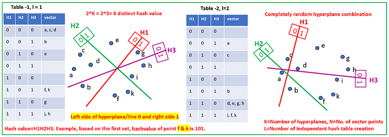
Hash Value Assignment For All Vector Points

Generate a series of random hyperplanes to partition the space.
Assign items to partitions, giving them the same hash value if they are in the same partition (see in the fig below, how hash value is assigned to each vector point).
For a dataset with N points and d dimensions: * Generate K random hyperplanes. * For each point, create a hash where the kth bit of the hash is 1 if the point is on one side of the kth hyperplane, and 0 if on the other.
Repeat the process L times with L different sets of K hyperplanes to construct L independent hash tables.

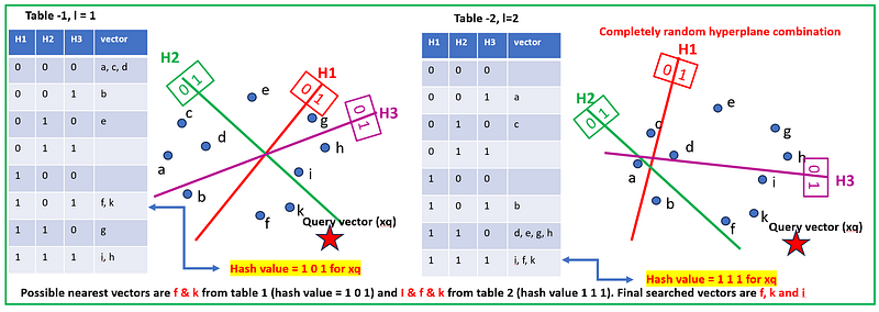
Similarity Search For Query Vector (xq): To conduct a similarity search for a new point with the LSH Random Projection technique, the process begins by generating a hash for the new point using predefined random hyperplanes, assigning bits based on the point’s position relative to these hyperplanes. This hash leads to a specific bucket in the hash table, where potential nearest neighbors — those with a high probability of similarity — are gathered. A detailed similarity check, such as cosine similarity or Euclidean distance, is then performed within this bucket to account for possible hash collisions. If multiple hash tables are in play, this process repeats for each to enhance the accuracy of the search. The subsequent step involves aggregating the potential neighbors from all hash tables, with points appearing in multiple buckets marked as highly similar. These candidates are then ranked by their computed similarity, and the top-ranking points are returned as the nearest neighbors to the new point, thus streamlining the nearest neighbor search in large, high-dimensional datasets.

Implementation of LSH Random Projection Method: The code snippet below demonstrates how to implement the Locality-Sensitive Hashing (LSH) Random Projection method using faiss. The approach taken by faiss differs slighlty from the one we discussed above, as it only incorporates a single hash table (l=1) in its implementation.

## Reading data file
import pandas as pd
import faiss
df=pd.read_csv('https://raw.githubusercontent.com/DhunganaKB/customchat/main/VectorIndexSearch/TextClassification_Indexing.csv')
df = df.reset_index(drop=True)

## Creating embedding vectors
from sentence_transformers import SentenceTransformer
model = SentenceTransformer('bert-base-nli-mean-tokens')
sentences = list(df['Sentence'])
sentence_embeddings = model.encode(sentences)
embedding_dimension = sentence_embeddings.shape[1]
print(embedding_dimension)

## Create index using faiss

# this tell us how many hyperplanes we want to consider,
nbits=4
#Here we choose 16 buckets or hash values = 2**4 = 1<<nbits
1<<nbits
#2**4
# index created
index = faiss.IndexLSH(embedding_dimension, nbits)
# added embedded vector in the index
index.add(sentence_embeddings)
# we want 3 similarity vectors 
k=3
# created query vector
xq=model.encode(['I would like to know about Nobel Prize from 2020'])

## make a similarity search

#xq = xq.reshape(1,embedding_dimension)
D, I = index.search(xq, k=k)

print(I)

# [[34  4 16]]

Production Quantization:

Product quantization for similarity search in vector space is a method that compresses high-dimensional vectors into shorter pieces by breaking them down into smaller, more manageable sub-vectors and quantizing each one. This approach retains enough information to allow the vectors to be compared for similarity. The term “manageable sub-vectors and quantizing each one” refers to two steps in the process of product quantization:

1. Creating Manageable Sub-Vectors: High-dimensional vectors (which are long lists of numbers that represent points in a multi-dimensional space) are divided into smaller, more manageable pieces. For example, if we have a vector with 100 dimensions, we might break it into 10 sub-vectors, each with 10 dimensions. These smaller sub-vectors are easier to work with because they require less computational resources to process.

2. Quantizing Each Sub-Vector: Once we have these sub-vectors, the next step is to quantize them. Quantization is a process where you map these sub-vectors to a predefined set of representative values, known as codebooks or centroids. Each centroid represents a cluster of sub-vectors that are close to each other in the space of possible values. Instead of storing the exact sub-vector, we store the index of the nearest centroid. This is a form of lossy compression because it reduces the precision of the sub-vector data, but in a controlled way that retains most of the information important for similarity searches.

Here’s how Production Quantization makes vector similarity search faster:

1. Storage Efficiency: Since vectors are compressed, they take up less memory, enabling faster data retrieval.

2. Computational Speed: It’s quicker to compare the short codes resulting from product quantization than to compare the original high-dimensional vectors.

3. Approximation: The method approximates the distance between vectors rather than calculating the exact distance, which reduces computation time.

4. Batch Processing: By quantizing vectors in parts, it allows for batch processing during the search, which can be done in parallel, speeding up the overall process.

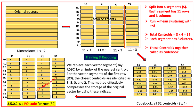
Training & Encoding

— The algorithm starts by taking the high-dimensional data and dividing it into smaller, more manageable subspaces — subvectors. — It then applies a clustering algorithm, typically k-means, to each subspace to find the ‘centroids’ or the representative points of the data clusters within that subspace. — These centroids form a codebook for each subspace, which is used to encode the data.

— Once the codebooks are established, each high-dimensional vector in the dataset is encoded by finding the nearest centroid in each subspace. — The original vector is then represented by a combination of these centroids’ indices, one from each subspace’s codebook. — This results in a compressed form of the dataset where vectors are replaced by a short code composed of the indices of the nearest centroids.

The training phase is crucial as it determines the quality of the centroids, which directly affects the accuracy of the encoding. The encoding phase is where the actual dimensionality reduction takes place, enabling efficient storage and retrieval of high-dimensional data. The points discussed above are visually represented in the image below.

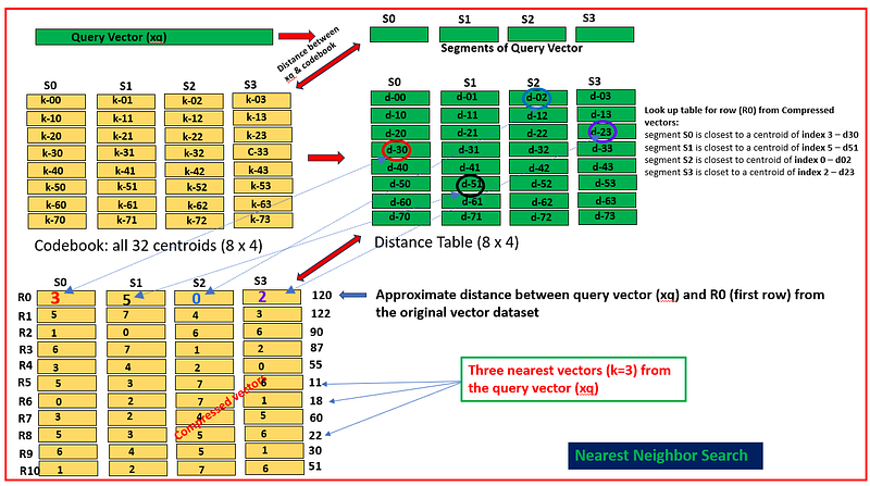
Nearest Neighbor Search:

Nearest neighbor search with PQ works efficiently by leveraging the compact representations (Compressed Vectors) of the data created during the PQ training and encoding. The optimized search procedure consists of the following steps:

— Split the query vector into subvectors, just as the database vectors are divided during the training phase. — For each subvector of the query vector, calculate the distance to all centroids within the corresponding subspace (codebook). These distances are referred to as partial distances. — Store the computed partial distances in a table, distance table. — To estimate the distance from the query vector to a database vector: — — Retrieve the partial distance from the distance table for each subvector of compressed vecor using its PQ code. — — Sum the squared partial distances to approximate the squared euclidean distance.

— The final step is to aggregate these partial distances. For Euclidean distance, this involves summing the squared partial distances and then taking the square root of the sum to obtain the approximate total distance.

— Once you have the approximate distances for all database vectors, you can sort them to find the nearest neighbors to the query vector.

The steps mentioned above are depicted visually in the following illustration.

Implementation of product quantization: The code snippet below demonstrates how to implement the product quantization method using faiss.

import pandas as pd
import faiss
pd.set_option('display.max_colwidth', 200)  # Adjust the width as needed
import faiss
df=pd.read_csv('https://raw.githubusercontent.com/DhunganaKB/customchat/main/VectorIndexSearch/TextClassification_Indexing.csv')
df = df.reset_index(drop=True)
df.head()
from sentence_transformers import SentenceTransformer
model = SentenceTransformer('bert-base-nli-mean-tokens')
sentences = list(df['Sentence'])
sentence_embeddings = model.encode(sentences) # embedded vector
embedding_dimension = sentence_embeddings.shape[1]
print(embedding_dimension)

m = 16 # dimention of each segment
assert embedding_dimension % m ==0
# define the number of cluster
nbits=4 # k = 2**nbits = 16 # since this data set is small
index = faiss.IndexPQ(embedding_dimension, m, nbits)

print(index.is_trained)
index.train(sentence_embeddings)
index.add(sentence_embeddings)
# query vector
xq=model.encode(['I would like to know about Nobel Prize from 2020'])
dist, I = index.search(xq, k=3)
print(I)
# [[22 28 20]]
# see those indexes from the original dataframe
df.iloc[I[0]]

The Product Quantization (PQ) method for similarity search offers a highly memory-efficient approach by compressing high-dimensional data into compact codes. While it introduces some lossiness due to quantization, the method still achieves a good balance between accuracy and efficiency, making it suitable for large-scale applications. PQ’s ability to perform fast approximate nearest neighbor searches by leveraging precomputed distances to centroids makes it a valuable technique in the field of information retrieval.

In conclusion, following our exploration of Flat, IVF, and HNSW methods for similarity search in our previous articles, we have now examined three additional ANN techniques: ANNOY, Random Projection LSH, and Product Quantization. These methods expand our toolkit for efficient similarity search in diverse datasets.

I hope you have found this article helpful. Thank you for taking the time to read it!

If there are any questions and would like to discuss, please don’t hesitate to get in touch with me via LinkedIn.

Refrences: