A Beginner’s Guide to Similarity Search & Vector Indexing (Part One)

Part 1, Part 2, and Part 3 of this series.

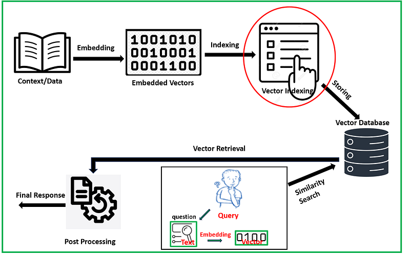
Similarity search in the context of Retrieval Augmented Generation (RAG) involves finding and retrieving relevant pieces of information or data points that are similar to a given query vector. RAG is an approach in generative AI that combines retrieval-based methods with generative models to enhance the quality and relevance of generated content. Vector indexing methods are techniques used to efficiently store, organize, and retrieve high-dimensional data points or vectors in databases and data structures. The choice of vector indexing method depends on various factors, including the dimensionality of the data, the trade-off between precision and recall, the size of the dataset, and the computational resources available. Different methods excel in different scenarios, so selecting the appropriate indexing method is crucial to achieving efficient and accurate search in high-dimensional vector spaces.

Similarity metrics: In RAG (Retrieval Augmented Generation), a similarity metric is a mathematical measurement used to evaluate how similar or relevant a query vector is to vectors in a dataset. This metric quantifies the degree of similarity or dissimilarity, guiding the RAG model in selecting the most pertinent data points for context-aware content generation. Most common similarity metrics are cosine similarity, inner product and euclidean distance. Two vectors representing words/sentences meanings may be “close” to one another if they are used in similar contexts or related to similar ideas. The detail explanation of similarity metrics can be found in these articles — one & two.

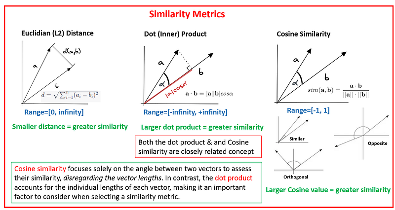
Cosine Similarity: It exclusively focuses on vector direction and evaluates the angle formed between two vectors. Cosine similarity is a metric that falls within the range of -1 to 1. A score of 1 indicates that the vectors are perfectly aligned (with a 0-degree angle), 0 signifies orthogonality (perpendicularity), and -1 suggests that the vectors are pointing in precisely opposite directions. In practical applications, we often use Cosine distance, which is calculated as 1 minus the Cosine similarity value (cosine distance = 1 — cosine similarity). This transformation extends the range from 0 to 2, where 0 denotes highly similar vectors, and 2 represents vectors that are diametrically opposed to each other. See the refrence.

Euclidean Distance: The Euclidean distance represents the direct, shortest distance between two vectors within a multi-dimensional space. Its values span from 0 to infinity. When the Euclidean distance is minimal, it indicates that the values of each coordinate in the vectors are closely aligned. A distance of zero signifies that the vectors are identical, while larger distances imply greater dissimilarity between them. See the refrence.

Inner (dot) Product: It quantifies the alignment between two vectors, with its value spanning from negative infinity to positive infinity. The dot product yields a higher value when the vectors are oriented in a similar direction, a smaller value when they point in opposite directions, and it becomes zero when they are orthogonal to each other.

The initial stage of this process (RAG) involves text embedding, where textual data is transformed into numerical vectors, each vector encapsulating specific semantic meaning. These embedded vectors serve as the foundation for our indexing process, enabling us to implement efficient similarity search using various similarity metrics.

In this article, I will explore two separate indexing techniques: Flat and IVF, while the exploration of additional methods will be covered in the second part. If you’d like to follow the steps provided in this article, you can find sample data and a Jupyter notebook in my GitHub repository.

Vector Indexing Methods

Flat Indexing: Flat indexing is a method of indexing wherein vectors are stored without any modifications, maintaining their original form. This approach is known for its simplicity, ease of implementation, and ability to deliver perfect accuracy. However, it does come with the drawback of being relatively slow in operation. In a flat index, the system calculates the similarity between the query vector and every other vector present, subsequently selecting the top k vectors with the highest similarity scores. Flat indexing is the ideal choice when very high precision is essential, and speed is not a primary concern. Additionally, for smaller datasets, flat indexing can still offer reasonable search speeds, making it a practical option in such cases. Let’s construct a flat index utilizing the faiss library.

import pandas as pd
import numpy as np
from sklearn.manifold import TSNE
import matplotlib.pyplot as plt
import seaborn as sns
from sklearn.cluster import KMeans
from scipy.spatial import Voronoi, voronoi_plot_2d
from federpy.federpy import FederPy
import faiss

## read data directly from the given link
df=pd.read_csv('https://raw.githubusercontent.com/DhunganaKB/customchat/main/VectorIndexSearch/TextClassification_Indexing.csv')
df = df.reset_index(drop=True)
df.shape # (109,2)

The initial stage involves generating embedding vectors, and the provided code snippet assists us in accomplishing this task.

from sentence_transformers import SentenceTransformer
model = SentenceTransformer('bert-base-nli-mean-tokens')

sentences = list(df['Sentence'])
sentence_embeddings = model.encode(sentences)
embedding_dimension = sentence_embeddings.shape[1]
print(embedding_dimension)

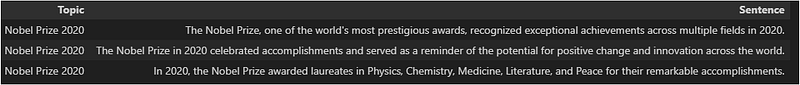
Next, let’s establish a flat indexing structure. We are utilizing the faiss library with the IndexFlatL2, which calculates the L2 (Euclidean) distance. The index.is_trained attribute indicates whether training is necessary before storing vectors in this indexing system. In this case, no prior training is needed; we can directly add embedding vectors to this indexing system. Following that, we define a query vector using the same embedding model with the intention of searching for the top 3 most similar vectors. The retrieved indexes correspond to 20, 28, and 22.

index=faiss.IndexFlatL2(embedding_dimension)
print(index.ntotal, index.is_trained)
## now adding embedding vector in sentence embeddings
index.add(sentence_embeddings)
print(index.ntotal)

xq=model.encode(['I would like to know about Nobel Prize from 2020'])

k=3
D, I = index.search(xq, k)  # search
print(I)

[[20 28 22]]

df.iloc[I[0]]

These sentences are derived from the indexes we retrieved.

Let’s attempt the same process without relying on the faiss library, and it will yield us identical indexes. Euclidean distance is utilized here.

## First measure distance 
distance=[]

for sub_array in sentence_embeddings:
    distance.append(euclidean(sub_array, xq[0]))


# finding the index of smallest values

def finding_index_smallvalue(lst, k):
    indexed_xx = list(enumerate(lst))

    # Sort the list of tuples based on the values (ascending order)
    sorted_xx = sorted(indexed_xx, key=lambda x: x[1])

    # Get the indices of the smallest three numbers
    smallest_indices = [i for i, value in sorted_xx[:k]]

    return smallest_indices

I=finding_index_smallvalue(distance, 3)
print(I)
[20, 28, 22]

We can also experiment with the inner product as a similarity measure. All of these approaches yield the same set of indexes as mentioned previously.

## using faiss library

index1=faiss.IndexFlatIP(embedding_dimension)
index1.add(sentence_embeddings)
D, I = index1.search(xq, k)  # search
print(I)

[[20 28 22]]

## without faiss
distance1=[]

for sub_array in sentence_embeddings:
    distance1.append(np.inner(sub_array, xq[0]))

def finding_index_largevalue(lst, k):
    indexed_xx = list(enumerate(lst))

    # Sort the list of tuples based on the values (ascending order)
    sorted_xx = sorted(indexed_xx, key=lambda x: x[1], reverse=True)

    # Get the indices of the smallest three numbers
    largest_indices = [i for i, value in sorted_xx[:k]]

    return largest_indices

I=finding_index_largevalue(distance1, 3)
print(I)
[[20 28 22]]

Now, let’s explore this graphically. Our embedded vector has a dimensionality of 768. In order to create a visual representation of this dataset, we employ the t-SNE method to map the embedding vectors into a 2-D space. As depicted below, there are a total of 109 vectors. In the first step, this method calculates the distances between the query vector and all 109 vectors, and subsequently, in the second step, it identifies the closest vectors.

The code snippet responsible for generating the visualization shown above is as follows:

plt.rcParams['figure.figsize'] = (12, 6) 

tsne = TSNE(n_components=2, perplexity=15, random_state=42, init='random', learning_rate=200)

vis_dims2 = tsne.fit_transform(sentence_embeddings)

x_values = [x for x,y in vis_dims2]
y_values = [y for x,y in vis_dims2]

plt.scatter(x_values, y_values)
for i, (x, y) in enumerate(zip(x_values, y_values)):
    plt.annotate(str(i), (x, y), textcoords="offset points", xytext=(0, 3), ha='center')

plt.title("Reduced Dimension: Embeddings visualized using t-SNE", size=17, fontweight="bold")
plt.xlabel('X1',size=13, fontweight="bold")
plt.ylabel('X2',size=13, fontweight="bold")

Approximate Nearest Neighbor (ANN)

Flat indexing, while straightforward, is often insufficient for efficient similarity search in large and high-dimensional datasets. As the dataset size increases, performing exact nearest neighbor search across all data points sequentially becomes computationally expensive and impractical. This is where ANN search methods come into play. ANN techniques strike a balance between search accuracy and computational efficiency, enabling us to quickly identify data points that are approximately similar to a query point, even if they are not the exact nearest neighbors. ANN algorithms optimize the search process by reducing the search space and using efficient data structures such as trees, hashes, graphs, or vector quantization.

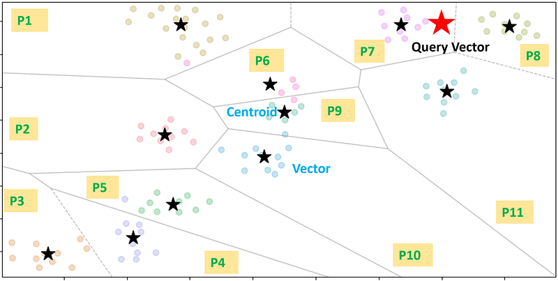
Inverted File (IVF) Indexing : This is one of the techniques used in Approximate Nearest Neighbor (ANN) search. It arranges data into partitions linked to centroids, simplifying the process of finding relevant data points during ANN searches. By structuring the entire dataset into partitions, an inverted file index narrows down the search space. Each partition is linked to a centroid, and every vector in the dataset is placed in a partition corresponding to its closest centroid.

Let’s employ the Faiss library to create an IVF (Inverted File with Flat) index. The “nlist” parameter determines the number of partitions we intend to establish. In this code, the “quantizer” is an instance of a basic flat index (“IndexFlatIP”), serving as the initial component within the IVF index structure. It quantizes input vectors and assists in organizing them into inverted lists, optimizing similarity searches in high-dimensional spaces using the inner product as the similarity metric. Initially, the index is untrained (“index.is_trained=False”), so we must first train it with the embedding vectors before adding them to the index. As indicated in the final line, it also identifies the same indexes as the nearest ones to the query vector. Additionally, we have configured “nprob=3”, specifying the number of partitions to include in our final search (out of the 11 available partitions, we select only 3).

nlist=11
quantizer = faiss.IndexFlatIP(embedding_dimension)
index = faiss.IndexIVFFlat(quantizer, embedding_dimension, nlist)
print(index.ntotal, index.is_trained)

index.train(sentence_embeddings)  # we must train the index to cluster into cells
index.add(sentence_embeddings)
index.nprobe=3
D, I = index.search(xq,3)
print(I)

[[20 28 22]]

I’d like to demonstrate how to generate these partitions using the k-means clustering method, allowing us to visualize the end result in a 2-D format. To achieve this, let’s begin by establishing clusters and then creating Voronoi cells based on these clusters. Given that this dataset encompasses 11 distinct topics, I’ve opted for “n_cluster=11”, but you can select a different number as needed.

## K-mean clustering
km_model = KMeans(n_clusters = nlist, init ='k-means++', random_state = 42)
y = km_model.fit_predict(sentence_embeddings)
df['Cluster']=y

# using TSNE library, we project our embedding vectors into 2-D

tsne = TSNE(n_components=2, perplexity=15, random_state=42, init='random', learning_rate=200)
vis_dims2 = tsne.fit_transform(sentence_embeddings)

x = [x for x,y in vis_dims2]
y = [y for x,y in vis_dims2]

palette = sns.color_palette("husl", nlist).as_hex()

lst=[]
for category, color in enumerate(palette):
    xs = np.array(x)[df.Cluster==category]
    ys = np.array(y)[df.Cluster==category]
    #plt.scatter(xs, ys, color=color, alpha=0.3, s=50)

    avg_x = xs.mean()
    avg_y = ys.mean()

    lst.append([avg_x, avg_y])
    
lst=np.array(lst)

Here, we’ve utilized the t-SNE method to project our embedded vectors into a 2-D space. Following this projection, we construct a Voronoi diagram.

vor = Voronoi(lst)

# Plot Voronoi diagram
voronoi_plot_2d(vor, show_vertices=False, show_points=False, line_colors='gray', line_width=1, line_alpha=0.5)

palette = sns.color_palette("husl", nlist).as_hex()

#lst=[]
for category, color in enumerate(palette):
    xs = np.array(x)[df.Cluster==category]
    ys = np.array(y)[df.Cluster==category]
    plt.scatter(xs, ys, color=color, alpha=0.3, s=50)

    avg_x = xs.mean()
    avg_y = ys.mean()

#    lst.append([avg_x, avg_y])
    
    plt.scatter(avg_x, avg_y, marker='*', color='black', s=300)

# plt.xlim(-120,120)

#plt.title("Reduced Dimension: Embeddings visualized using t-SNE", size=17, fontweight="bold")
plt.xlabel('X1',size=13, fontweight="bold")
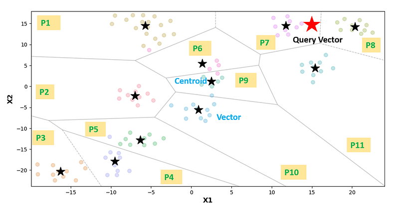
plt.ylabel('X2',size=13, fontweight="bold")

As observed below, it’s evident that there exist 11 partitions in the Voronoi diagram, each with its centroid. During a query search within this space, the process involves initially computing the distances between the query vector and all centroids, selecting a subset of partitions (in this case, 3) that are closest to the query vectors. Subsequently, it calculates the distances between the query vector and all other vectors from the chosen partitions and selects the closest vectors among them. This approach significantly reduces the search space, resulting in a highly efficient process.

Visualization Using Federpy: Feder is a JavaScript tool designed to aid in the comprehension of embedding vectors. It visualizes index files from Faiss, HNSWlib, and other ANN libraries to provide insight into how these libraries function and the concept of high-dimensional vector embeddings. Feder is written in javascript, and also provide a python library federpy, which is based on federjs.

To achieve this, we need to save the index file first. The provided code snippet enables us to visualize the IVF index generated using the faiss library. It’s worth noting that in cases where the number of partitions is low, there may be occasional difficulties in generating the visualization. Here, I’ve selected 20 partitions and set “nprobe=5”.

## For visualization of 
nlist=20
index = faiss.index_factory(embedding_dimension, 'IVF%s,Flat' % nlist)
index.train(sentence_embeddings)
index.add(sentence_embeddings)
index.nprobe = 5
faiss.write_index(index, 'faiss_ivf_flat_sample.index')

ivfflatSource = 'faiss'
ivfflatIndexFile = 'faiss_ivf_flat_sample.index'
federPy_ivfflat = FederPy(ivfflatIndexFile, ivfflatSource)
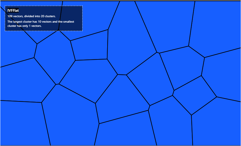
federPy_ivfflat.overview()

Here’s what the Voronoi diagram looks like for this dataset, illustrating a total of 109 vectors distributed among 20 partitions.

We have the option to perform searches based on either the ID or the query vector.

federPy_ivfflat.searchById(22)
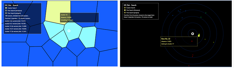
federPy_ivfflat.setSearchParams({"k": 3, "nprobe": 5}).searchByVec(xq[0])

The visuals are interactive, enabling us to retrieve the indexes and distances of the nearest vectors in relation to the query vector. This visualization provides valuable insights into the position of the query vector, along with the indexes and distances of its closest neighboring vectors, making it a valuable tool for understanding the data points.

Please don’t hesitate to give it a try. You can explore the complete Jupyter notebook for such visuals by accessing it at this link.

In this article, we have provided a concise overview of similarity metrics and introduced two vector indexing techniques. It’s important to note that the field of Approximate Nearest Neighbors (ANN) encompasses several additional methods that we haven’t had the opportunity to delve into within this article. You can look forward to a deeper exploration of these methods in Part 2, where we will expand upon and discuss their relevance in more detail. Stay tuned for a comprehensive exploration of the full spectrum of ANN techniques in the upcoming installment.

I hope you have found this article helpful. Thank you for taking the time to read it!

If there are any questions and would like to discuss, please don’t hesitate to get in touch with me via LinkedIn.