YOLO v4 explained in full detail

For this story, we will take a deep look into the YOLOv4, the original paper is huge and has a ton of things. So, fasten your seat belts as it is going to be an extremely long blog to follow just because of the sheer number of things presented in the YOLOv4 paper. All the YOLO models are object detection models, and with the release of YOLOv4, there is a significant increase in the inference time of the model. It can be trained on a single GPU as that is what the authors initially set out to do.

I’m assuming that you know how YOLO works for those who want to know it in more detail can look here.

YOLOv4 is very complex and that’s why this blog is to understand the advancement made over the original YOLO. So, without further ado let’s unwrap YOLOv4 in different sections.

• Object detector architecture breakdown
• Backbone, neck, head
• Bag of freebies (BoF)
• Bag of specials (BoS)
• YOLOv4 architecture selection
• YOLOv4 BoF and BoS selection

Object detector architecture breakdown

The original YOLO (You Only Look Once) was written by Joseph Redmon in a custom framework called Darknet. Darknet is a very flexible research framework written in low-level languages and has produced a series of the best real-time object detectors in computer vision: YOLO, YOLOv2, YOLOv3, and now, YOLOv4.

The Original YOLO — YOLO was the first object detection network to combine the problem of drawing bounding boxes and identifying class labels in one end-to-end differentiable network.

YOLOv2 — YOLOv2 made a number of iterative improvements on top of YOLO including BatchNorm, higher resolution, and anchor boxes.

YOLOv3 — YOLOv3 built upon previous models by adding an objectness score to bounding box prediction, added connections to the backbone network layers and made predictions at three separate levels of granularity to improve performance on smaller objects.

Now on to the YOLOv4, it is a one-stage detector with several components to it. Each component will be broken down further in the later section of the blog.

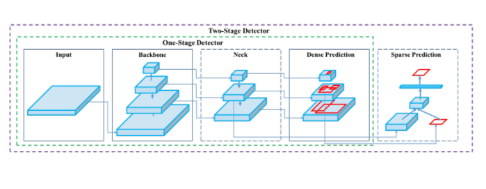
Here are the different building blocks of YOLOv4.

Input: Image, patches, Pyramid

Backbone: VGG16, ResNet-50, SpineNet, EfficientNet-B0-B7, CSPResNext50, CSPDarknet53.

Neck:

• Additional Blocks: SSP, ASPP, RFB, SAM
• Path-aggregation blocks: FPN, PAN, NAS-FPN, Fully-connected FPN, BiFPN, ASFF, SFAM

Heads:

• Dense prediction (one-stage):

1. RPN, SSD, YOLO, RentinaNet (anchor-based)
2. CornerNet, CenterNet, MatrixNet (anchor-free)

• Sparse prediction:

1. Faster R-CNN, R-FCN, Mask R-CNN (anchor-based)
2. RepPoints (anchor-free)

You can see that YOLOv4 can be implemented in any combination of input, backbone, neck, and head.

Backbone, neck, head

Backbone is the deep learning architecture that basically acts as a feature extractor. All of the backbone models are basically classification models. I assume that everyone is familiar with at least VGG16. One of the earliest deep learning classifiers. There are three more models that we can use in the backbone other than the models mentioned above namely SqueezeNet, MobileNet, ShuffleNet, but all of them are meant for CPU training only.

Neck is a subset of the bag of specials, it basically collects feature maps from different stages of the backbone. In simple terms, it’s a feature aggregator. The neck of the object detection pipeline will be discussed in more detail in later sections.

Head is also known as the object detector, it basically finds the region where the object might be present but doesn't tell about which object is present in that region. We have two-stage detectors and one stage-detectors which are further subdivided into anchor-based and anchor-free detectors. Head will be discussed in more detail in the later sections.

Bag of freebies (BoF)

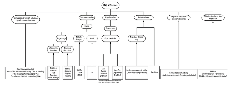
Bag of freebies are those methods that only change the training strategy or only increase the training cost (nothing to do with inference). You can see from the above diagram that there are an insane amount of things you can try, but we will discuss only the most important ones.

Bag of specials (BoS)

Bag of specials are those Plugin modules and post-processing methods that only increase the inference cost by a small amount but can significantly improve the accuracy.

Now we have dealt with all the components present in YOLO, let’s understand all the components in more detail.

YOLOv4 architecture selection

As we have seen that there are a lot of possibilities in choosing the architecture. So, what exactly do we look for while choosing the architecture? Selection criteria are based on the optimal balance between input network resolution (input image size), number of convolution layers, number of parameters, and number of output layers (filters). Also, we have an additional block for increasing the receptive field (bag of specials) and the best method from different backbone levels to different detector levels (Necks).

The final architecture presented in the paper is

CSPDarkNet53 (Backbone) => SSP + PANet (Neck)=> YOLOv3 (head)

Other close competitors were CSPResNext50 and EfficientNet-B3 but CSPDarkNet gave a higher FPS than the rest.

Generally, more parameters or BFLOPS mean less FPS but that is not the case here definitely. So, that’s why the authors choose CSPDarkNet53.

There is one important thing to be discussed before we discuss SSP and PANet and it is the effect of the resolution. In contrast to the classifier, the detector requires a higher input network size for detecting multiple small-sized objects. It also needs more layers for a higher receptive field to cover the increased size of the input network. In short, it needs more parameters for the greater capacity of a model to detect multiple objects of different sizes in a single image.

The impact of receptive field size

The influence of the receptive field with different size

• Up to the object size — allows viewing the entire object
• Up to the network size — allows viewing the context around the object
• Exceeding the network size — increases the number of connections between the image point and the final activation

YOLOv4 BoF and BoS selection

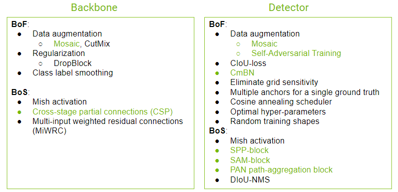
Let’s discuss the highlighted sections of the above image.

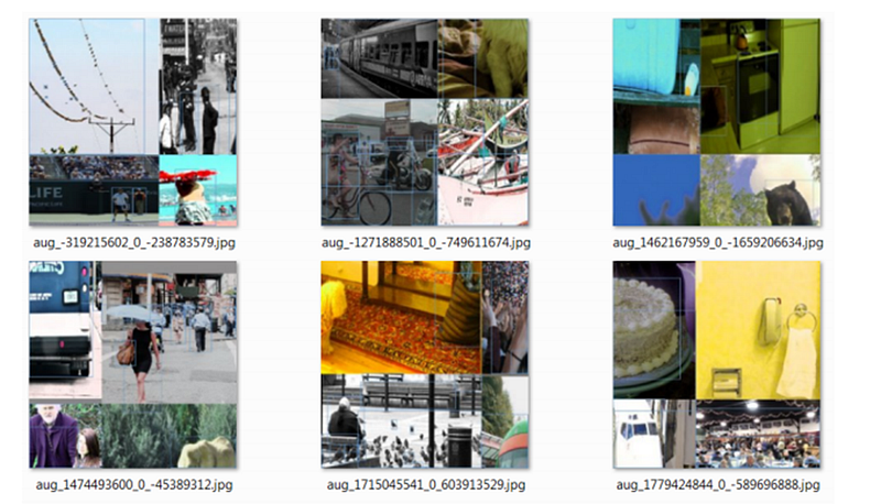
Mosaic

• Allows detection of objects outside their normal context
• Batch normalization calculates activation statistics from 4 different images -> reduce the need for large mini-batch size

Self-Adversarial Training (SAT)

We know that DL performs super bad with adversarial data and thus YOLOv4 uses SAT such that it introduces the X amount of perturbation to the training data till the predicted label remains the same as the original class. This helps the model to become more generalized.

If you want to know more about the effect of adversarial attacks on DL:

CSP: Cross-Stage Partial Connection

As the number of layers grows, the last layers have a lesser and lesser context of the features learned in the initial layers. In order to solve that researchers introduced the idea of skip connections such that the gradient can backpropagate to the initial layers with relative ease. DenseNet was one such network, that has skip connections from every layer to another. But the problem with DenseNet is that it has too many parameters, making it harder to train and do inference. The CSPResNext50 and the CSPDarknet53 are both based on DenseNet.

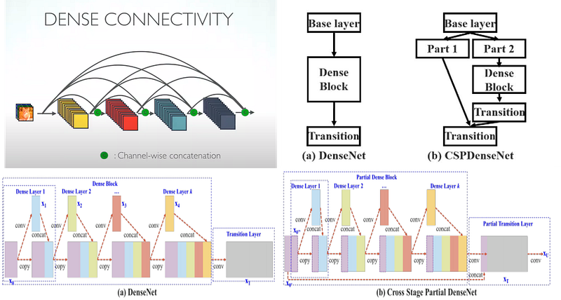
In CSPResNext50 and CSPDarknet53, the DenseNet has been edited to separate the feature map of the base layer by copying it and sending one copy through the dense block and sending another straight on to the next stage. The idea with the CSPResNext50 and CSPDarknet53 is to remove computational bottlenecks in the DenseNet and improve learning by passing on an unedited version of the feature map. Cross-stage partial connection was tried on ResNext-50 and there was a massive increase of around 20%

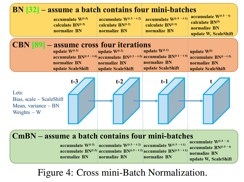
CmBN: Cross-Iteration mini Batch Normalization

I assume that all of you know about Batch Normalisation, so cross-batch normalization is normalizing the data with 4 batches in training. So, during the training data is passed as a batch and the entire batch is normalized but it has no correlation with the previous batch or batch coming after it. CBN takes into account the mean and standard deviation of the past 4 batches and uses that to normalize the current batch. CmBN takes it even a step further, it introduces the idea of CBN in a single batch with mini-Batch normalization.

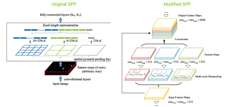
SPP: Spatial Pyramid pooling

YOLOv4 uses an SPP block after CSPDarknet53 to increase the receptive field and separate out the most important features from the backbone. Spatial pyramid pooling is that we take an input image and use Conv layers to extract its feature map, then use the max pool of window size_1 to generate a feature set, then again use the max pool of window size_2, repeat this n times and you will have different feature maps in height and width dimension, thus you make a pyramid. YOLOv4 takes this to the next step, instead of applying SPP it divides the feature along depth dimension, applies SPP on each part, and then combines it again to generate an output feature map.

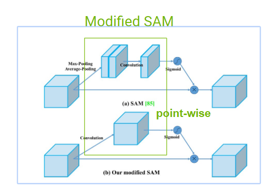
SAM: Spatial Attention Module

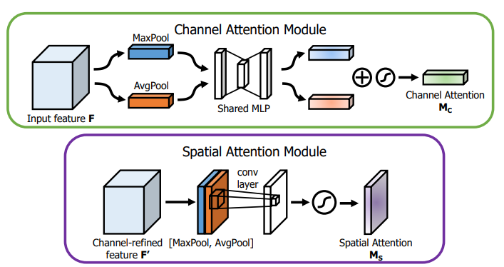
In order to understand the Special attention Module, we need to understand SENet (Squeeze and Excitation Network). What SENet basically does is find which channel is more important and which is less important in a feature map block. In the below diagram, you see a colored feature block that basically tells the importance of each filter in the feature map.

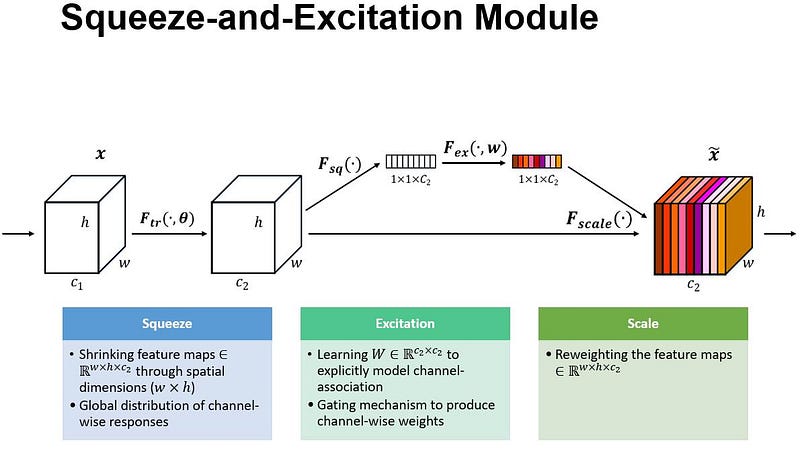
Now coming back to the SAM, we don’t squeeze each filter to a point rather use both max pool and average pool thus we get a reduced size (width and height wise) feature block which is fed to a sigmoid activation and then crosswise multiplied to the original feature map in order to obtain the feature importance of each filter in the feature map. So, this attention mechanism is along the depth/filter, but YOLOv4 again goes to a crazy level and applies the attention along width and height that is called spatial attention. It basically uses an attention mechanism along with both filters (depth) and spatial (width and height)

PAN Path — Aggregation Block

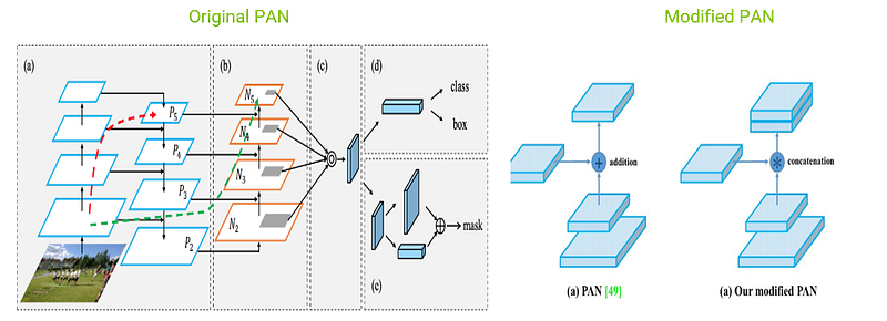
YOLOv4 chooses PANet for the feature aggregation of the network. They don’t write much on the rationale for this decision, and since NAS-FPN and BiFPN were written concurrently, this is presumably an area of future research. The thing that they modified in the YOLOV4 is that instead of using addition in the original PAN, they used concatenation. PANet is basically a Feature pyramid network that extracts important features from the backbone classifier. It uses SPP to make this FPN possible.

Wuff... finally we came to the end of this insanely long but interesting blog. The original paper is huge and very tough to grasp just because of the sheer number of things presented in the paper. We are not going to discuss the results and experimentation of the original paper, but know this it is still very close to the current state of the art.

If you want to check out more about object detection libraries and algorithms you can also look up Neptune.ai blog.

Thanks for giving your time and if you think that this blog added something to your knowledge base, please consider following the AI guys Blog and if you are interested to become a writer at AI guys you can follow this link.