
Role of Choosing Correct Loss Function
Loss functions play a very important role in the training of modern Deep learning architecture, choosing the right loss function is the key to successful model building. A loss function is a mathematical equation that a deep learning architecture tries to minimize or optimize. Deep learning is an iterative process, in every step, it calculates some metric that tells the system how close its prediction is to the original label. Based on the calculated loss value, the network optimizes its parameters. There are a lot of loss functions and among those, the most popular ones are Mean square error, categorical cross-entropy, Dice loss, etc. If you want to read more about different loss functions go to the TensorFlow website https://www.tensorflow.org/api_docs/python/tf/keras/losses
Loss functions can be divided into two major categories: specialized loss functions and generalized loss functions. Generalized loss functions are those functions that can be used with almost any DL task like text prediction, image recognition, image classification, etc (Mean square error). Whereas specialized loss functions are designed for specific applications like semantic segmentation. Boundary loss and focal loss are good examples of specialized loss functions. Before we move further, here’s a question to you, why do loss functions behave differently? Why are certain losses good for a particular task and bad for others?
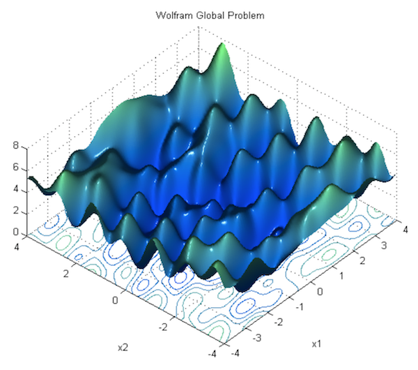
When I change the loss function, basically the optimization problem changes and that’s why we have different results. But the question remains, what exactly changed in the network’s learning? I can train a network with the same data and it will perform differently for different losses even if it gives the same accuracy. What exactly changes in the learning capacity of the network, you still have the same number of parameters, you still have the same connections among the neurons then what exactly has changed? The answer is very simple it’s the optimization surface has changed. Optimization surface is an N-dimensional space in which the network tries to find the global minima. Through the adjustment of weights and biases, the neural network optimizes the decision boundary such that it can better separate between different class points and in doing so it moves to different locations in the optimization surface.
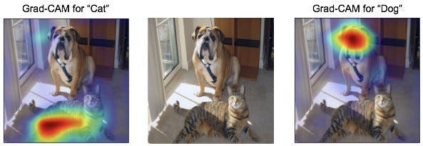
Before we move to the result section, let’s understand the internal working of neural networks. Through iterative training, the neural network starts identifying salient patterns hidden deep in the image. When we change the loss functions for a given deep learning architecture, what neural network finds salient also change. In simpler terms, what neural networks consider important to classify the data changes based on the loss function. Not every point in the image or datastream is of equal importance for the network to make its decision. For instance, if you train a dog classifier, the network weights will be modified to focus on identifying the dog’s face and for cats, they will be geared towards identifying their fur. If you look at the below image, you will understand what is saliency for the neural network. For dogs, their face is the most salient part and for the cats, their fur is the most salient part. Heatmap color shows the importance of different regions while making the final decision, red corresponds to the most important region for both the Dog and Cat class.
Let’s look at a few more saliency heatmaps. Given below is the gradients or salient part of a network trained to identify the hippocampus in the brain. The left image is generated through Binary Cross entropy and the right image is from the training of the same network with Dice loss.
BCE: https://en.wikipedia.org/wiki/Cross_entropy Diceloss:https://en.wikipedia.org/wiki/S%C3%B8rensen%E2%80%93Dice_coefficient
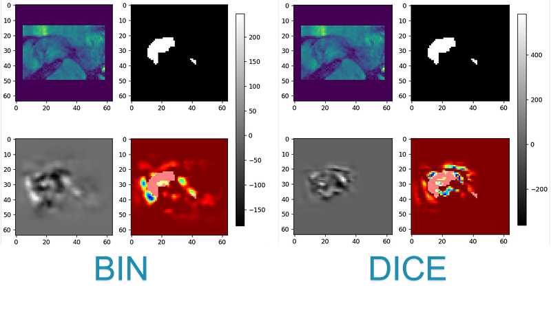
There are two key things to be noted from the above image, firstly, the scale of the gradients, secondly, the distribution of the gradient.
- If we look at the distribution of the gradients for the model trained with BCE, we see that active gradients have a spread over a much larger region compared to the active gradients of the model trained with Dice loss.
- Another difference is in the scale of gradients for both images, Dice has a much sharper transition from active to inactive gradients compared to BCE.
But why bother with this utter nonsense, why look into the gradients and their saliency?
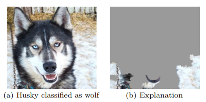
It is super important to know about saliency to make the models robust against adversarial attacks and also to know whether the model is looking into the right region or not while making its decision. The below image shows how a model can be completely off while making its decision. This model was performing at 90% accuracy for classifying the wolves and huskies but it was looking at the snow or no snow instead of the animal to classify the images of wolves.
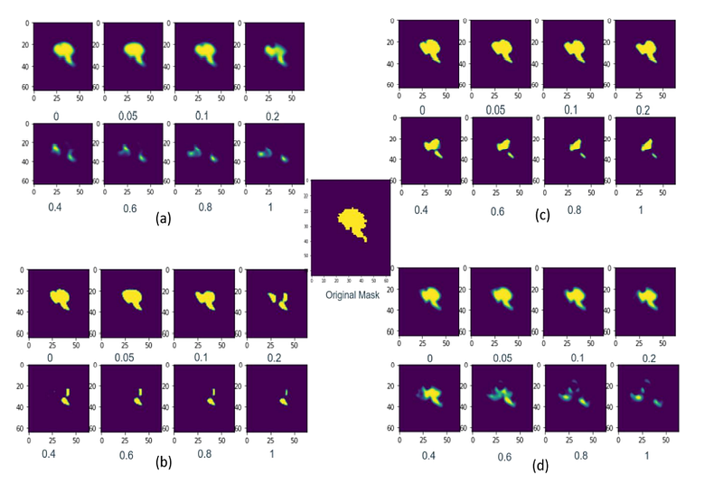
Let’s again look at the below image of hippocampus segmentation, we train 4 different models using (a) BCE, (b) Dice loss, (c) BCE+Dice, (d) BCE+Dice+Focal. To test their robustness performance we add noise to the pixels with the highest corresponding gradients. We added different intensity noise to 5 pixels only. This much noise is almost unrecognizable for the human eye.
We see that (c) BCE+Dice, (d) BCE+Dice+Focal are able to keep their segmentation mask for higher intensity noise compared to (a) BCE and (b) Dice loss. For the noise level of 2–5 times the maximum pixel value, the segmentation mask is almost gone.
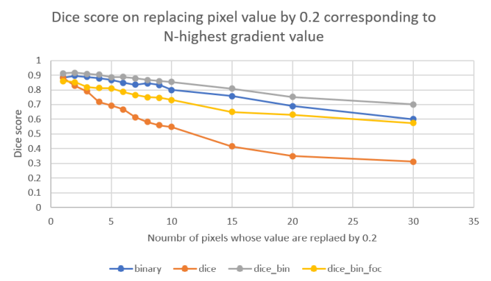
To put everything in numbers, look at the graph below, why choosing a correct loss function is super important. Your performance reduces from 90% to 30% just by changing the 5 most salient pixels in the input image. All the tests were performed on U-net.
I know this blog is a little complex and is written for people who are a little advance in the subject matter. Here’s the summary of all the experiments I carried out over a year.
- Dice loss gives us more accurate results for segmentation compared to BCE.
- It can be said with confidence that combining BCE and Dice loss gives the best result in terms of segmentation, pixel-wise accuracy, generalization, and performance against adversarial attacks.
- Changing a few pixels is enough to render the models with skip connections useless. Using specialized loss functions can force the network to focus very hard on very few pixels thus making them susceptible to adversarial attacks.
- BCE is much more resilient to both the level of noise and the number of pixels changed.
- The accuracy of models trained with different loss functions might be similar but what they look at and what they consider important might be different.
- At last, combining loss functions is a very good idea for training better and more robust models.
I know there’s a lot to chew in this blog, so people who want to explore this in more detail can look at my original research paper from which this blog is inspired. https://arxiv.org/abs/2110.08322


