X-Learner Uplift Model in Python

Manually create meta-learner X-learner: Model data processing, model training, prediction, individual treatment effect (ITE) and average treatment effect (ATE) calculation, and customer segmentation

X-learner is a meta-learner that is an extension of the T-learner. Compared with T-learner, X-learner is better for highly imbalanced treatment and control groups. In this tutorial, we will talk about the following:

• How to implement X-learner manually in Python?
• How to make an individual treatment effect (ITE) estimation using X-learner?
• How to calculate average treatment effect (ATE) estimation using X-learner?

Resources for this post:

• Video tutorial for this post on YouTube
• Click here for the Colab notebook.
• More video tutorials on Uplift Modeling
• More blog posts on Uplift Modeling

Let’s get started!

Step 0: X-learner Algorithm

X-learner consists of three stages, and each stage has model(s) that estimates different dependent variables.

• Stage one is the same as the T-learner. It builds two machine learning models to predict the outcomes, one using the treated units and the other using the control units.
• After the stage one models are built, the imputed individual treatment effect (ITE) will be calculated.

1. For the samples that received treatment, the imputed individual treatment effect (ITE) is the actual outcome minus the counterfactual outcome predicted by the control model from stage one.
2. For the samples that did not receive treatment, the imputed individual treatment effect (ITE) is the counterfactual outcome predicted by the treated model from stage one minus the actual outcome.

• Stage two builds two machine learning models to predict the imputed individual treatment effect (ITE), one model is trained using the treated units, and the other model is trained using the untreated units.
• After the stage two models are completed, the imputed individual treatment effect (ITE) predictions will be calculated separately using the treated and the control model for all the samples.
• Stage three builds a propensity model to predict the propensity of getting treatment. The predicted propensity score is used as the weight for the individual treatment effect (ITE) calculation.
• Finally, the individual treatment effect (ITE) will be estimated by getting the weighted average of the stage two model predictions, using the propensity scores as the weights.

To learn how to make an individual treatment effect (ITE) using a T-learner, please check out my previous tutorial T-Learner Uplift Model for Individual Treatment Effect (ITE) in Python.

Step 1: Install and Import Libraries

In step 1, we will install and import the python libraries.

Firstly, let’s install causalml for synthetic dataset creation.

# Install package
!pip install causalml

After the installation is completed, we can import the libraries.

• pandas and numpy are imported for data processing.
• synthetic_data is imported for synthetic data creation.
• seaborn is for visualization.
• LGBMRegressor and XGBClassifier is for the machine learning model training.

# Data processing
import pandas as pd
import numpy as np

# Create synthetic data
from causalml.dataset import synthetic_data

# Visualization
import seaborn as sns

# Machine learning model
from lightgbm import LGBMRegressor
from xgboost import XGBClassifier

Step 2: Create Dataset

In step 2, we will create a synthetic dataset for the X-learner uplift model.

• Firstly, a random seed is set to make the synthetic dataset reproducible.
• Then, using the synthetic_data method from the causalml python package, we created a dataset with five features, one treatment variable, and one continuous outcome variable.
• After that, the dataset is saved in a pandas dataframe.
• Finally, using value_counts on the treatment variable, we can see that out of 5000 samples, 2582 units received treatment and 2418 did not receive treatment.

# Set a seed for reproducibility
np.random.seed(42)

# Create a synthetic dataset
y, X, treatment, _, _, _ = synthetic_data(mode=1, n=5000, p=5, sigma=1.0)

# Save the data in a pandas dataframe
df = pd.DataFrame({'y': y, 'X1': X.T[0], 'X2': X.T[1], 'X3': X.T[2], 'X4': X.T[3], 'X5': X.T[4], 'treatment': treatment})

# Check treatment
df['treatment'].value_counts()

Output:

1    2582
0    2418
Name: treatment, dtype: int64

Step 3: X-learner Model Data Processing

In step 3, we will process the data for the X-learner.

• Firstly, the dataset df is split into two datasets based on the value of the treatment variable. The treated units are saved in a dataframe called df_treated and the control units are saved in a dataframe called df_control.
• Then the feature matrix and the outcome variable are created for the treated and control dataframes separately. Features include X1, X2, X3, X4, and X5. The dependent variable(a.k.a. label) is the outcome column y. The names of the features are features_treated and features_control, and the names of the outcomes are y_treated and y_control.
• Finally, we checked the shape of the modeling data for the two models. The treated model has 2582 records and the control model has 2418 records.

# Keep only the treated units
df_treated = df[df['treatment'] == 1]

# Features
features_treated = df_treated[['X1', 'X2', 'X3', 'X4', 'X5']]

# Dependent variable
y_treated = df_treated[['y']]

# Print data shape
print(f'The feature maxtrix for the treated has {features_treated.shape[0]} records and {features_treated.shape[1]} features.')
print(f'The dependent variable for the treated has {y_treated.shape[0]} records.')

# Keep only the control units
df_control = df[df['treatment'] == 0]

# Features
features_control = df_control[['X1', 'X2', 'X3', 'X4', 'X5']]

# Dependent variable
y_control = df_control[['y']]

# Print data shape
print(f'The feature maxtrix for the control has {features_control.shape[0]} records and {features_control.shape[1]} features.')
print(f'The dependent variable for the control has {y_control.shape[0]} records.')

Output:

The feature maxtrix for the treated has 2582 records and 5 features.
The dependent variable for the treated has 2582 records.
The feature maxtrix for the control has 2418 records and 5 features.
The dependent variable for the control has 2418 records.

We also need the features for all the samples for the model predictions, and we gave it the name of features.

# Features for all the samples
features = df[['X1', 'X2', 'X3', 'X4', 'X5']]

Step 4: X-Learner 1st Stage Models on Outcomes

In step 4, we will train the X-learner stage one models. Two machine learning models will be built to predict the outcomes, one model using the treated units and the other model using the control units.

The model selection and hyperparameter tuning are important for the performance of an X-learner model. This is because the model performance affects the model predictions hence the accuracy of the individual treatment effect (ITE) estimation.

Many machine learning model algorithms can be used to build the X-learner models. The model algorithms include but are not limited to LASSO regression, Ridge regression, random forest, XGBoost, and a neural network model.

A light GBM model is used in this example, and the process is the same for other machine learning model algorithms. The models for the three stages of X-learner can use different machine learning algorithms.

Using the LGBMRegressor method, we fit the two X-learner stage one models using the features and the outcome variable for the treated and the control group separately.

# X-learner stage one model for the treated
s1_treated = LGBMRegressor().fit(features_treated, y_treated)

# X-learner stage one model for the control
s1_control = LGBMRegressor().fit(features_control, y_control)

Step 5: X-Learner 1st Stage Model Predictions on Outcomes

In step 5, we will make predictions using the X-learner stage one models to get the counterfactual outcome predictions.

To make the treatment effect estimation, two separate predictions need to be made using the trained stage one models:

• In the first prediction, the treated model is used for the prediction of the control group. This gives us the predicted outcome values if the control group received the treatment.
• In the second prediction, the control model is used for the prediction of the treatment group. This gives us the predicted outcome values if the treatment group did not receive the treatment.

# Predictions on the control group using the treated model
s1_treated_predict = s1_treated.predict(features_control)

# Predictions on the treated group using the control model
s1_control_predict = s1_control.predict(features_treated)

Step 6: X-Learner 2nd Stage Models on Imputed ITE

In step 6, we will train the second-stage models on the imputed individual treatment effect (ITE).

The imputed individual treatment effects (ITE) are calculated for the treatment group and the control group separately.

• For the treated group, the imputed individual treatment effect (ITE) is calculated by using the actual outcome minus the counterfactual outcome predicted by the first-stage control model.
• For the control group, the imputed individual treatment effect (ITE) is calculated by using the counterfactual outcome predicted by the first-stage treated model minus the actual outcome.

# Create a column for the predicted outcomes
df_treated['predicted_outcome'] = s1_control_predict

# Create a column for the imputed ite
df_treated['imputed_ite'] =  df_treated.apply(lambda row: row.y - row.predicted_outcome, axis = 1)

# Create a column for the predicted outcomes
df_control['predicted_outcome'] = s1_treated_predict

# Create a column for the imputed ite
df_control['imputed_ite'] =  df_control.apply(lambda row: row.predicted_outcome - row.y, axis = 1)

After getting the imputed individual treatment effect (ITE), we will run the second stage X-learner models. In the second stage models, the dependent variable is the imputed individual treatment effect (ITE), and the features are the five covariates.

Two models will be built to predict the imputed individual treatment effect (ITE), one using the treated group and the other using the control group.

# Light GBM model for the treated
s2_treated = LGBMRegressor().fit(features_treated, df_treated['imputed_ite'])

# Light GBM model for the control
s2_control = LGBMRegressor().fit(features_control, df_control['imputed_ite'])

Step 7: X-Learner 2nd Stage Model Predictions on Imputed ITE

In step 7, we will use the X-learner second-stage models to predict the imputed individual treatment effect (ITE).

Two values will be predicted for each unit in the dataset, one using the second-stage treated model and the other using the second-stage control model. The prediction results are saved in the dataframe that includes both the treated and the control units.

# Predictions using the treated model
s2_treated_predict = s2_treated.predict(features)

# Save the prediction results as a colum in the dataframe
df['s2_treated_predict'] = s2_treated_predict

# Predictions using the control model
s2_control_predict = s2_control.predict(features)

# Save the prediction results as a colum in the dataframe
df['s2_control_predict'] = s2_control_predict

Step 8: X-Learner Propensity Score Model

In step 8, we will build a propensity score model to predict the propensity of getting the treatment.

The dependent variable is the treatment, which has two values, 0 represents the untreated unit and 1 represents the treated unit. The predictors are the five features.

We can use any binary classification model to do the prediction. In this example, we will use XGBoost to illustrate the process. Please see my previous tutorial Hyperparameter Tuning For XGBoost for more details about the XGBoost model.

# Train the XGBoost model
xgb = XGBClassifier(seed=0).fit(features,df[['treatment']])

# Make predictions
xgb_predict_prob = xgb.predict_proba(features)[:,1]

# Save the prediction results as a colum in the dataframe
df['treatment_propensity_score'] = xgb_predict_prob

Step 9: X-learner Individual Treatment Effect (ITE)

In step 9, we will use X-learner to calculate the individual treatment effect (ITE).

X-learner individual treatment effect (ITE) is the weighted average of the second-stage predictions on the imputed individual treatment effect (ITE).

The authors of the X-learner paper suggested using the propensity score as the weights when the treatment group and the control group have similar sizes.

When the treated group is very large or very small compared with the control group, we can use 0 or 1 as weights to utilize the model results with the larger size.

Since our dataset is relatively balanced between the treatment and the control group, we will use the propensity score as the weight.

• The weights for the second-stage control model predictions are the propensity scores and the weights for the second-stage treated model predictions are 1 minus the propensity scores.
• When there are a lot of control units and only a few treated units, most units have low propensity scores, so the second-stage treated model gets more weight. Because the second-stage treated model is based on the first-stage control predictions, we are utilizing a model that has more data.
• Similarly, when there are a lot of treated units and only a few control units, most units have high propensity scores, so the second-stage control model gets more weight. Because the second-stage control model is based on the first-stage treated predictions, we are utilizing a model that has more data.

If you would like to learn more details about the intuitions behind the X-learner, please refer to the paper Meta-learners for Estimating Heterogeneous Treatment Effects using Machine Learning.

After calculating the individual treatment effect (ITE), the data is saved in a dataframe.

# Calculate the weighted ITE
df['ITE'] = df.apply(lambda row: row.treatment_propensity_score*row.s2_control_predict + (1-row.treatment_propensity_score)*row.s2_treated_predict, axis=1)

# Take a look at the data
df.head()

The histogram visualization of the individual treatment effect (ITE) shows a normal distribution.

• The average treatment effect is around 0.5.
• Most individuals in the dataset have a positive treatment effect.
• Some individuals have negative treatment effects.

# visualization
df.hist(column ='ITE', bins=50, grid=True, figsize=(12, 8))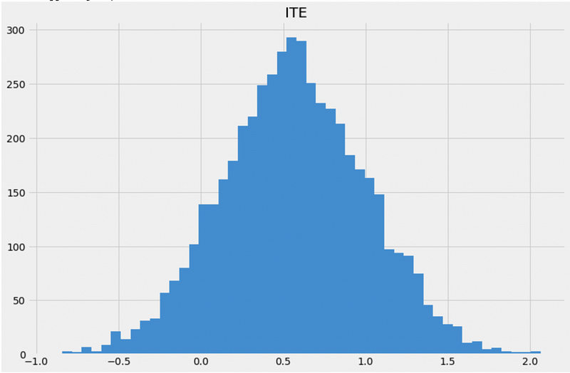

Step 10: X-Learner Average Treatment Effect (ATE)

In step 10, we will estimate the average treatment effect (ATE) using the X-learner predictions.

The average treatment effect (ATE) for the population is the average of the individual treatment effect (ITE). We can see that the average treatment effect (ATE) is 0.57.

To learn more about the definition and calculation for the average treatment effect (ATE), please check out my previous tutorial ATE vs CATE vs ATT vs ATC for Causal Inference.

# Calculate ATE
ATE = df[['ITE']].mean()

# Print out results
print(f'The average treatment effect (ATE) is {ATE[0]:.2f}')

Output:

The average treatment effect (ATE) is 0.57

Step 11: Customer Segmentation Using X-learner Individual Treatment Effect (ITE)

The customer segmentation using individual treatment effect (ITE) from the X-learner is the same as the T-learner and the S-learner. For the details about how to segment customers, please check out my previous tutorial S Learner Uplift Model for Individual Treatment Effect and Customer Segmentation in Python.

More tutorials are available on GrabNGoInfo YouTube Channel and GrabNGoInfo.com.

Recommended Tutorials

• GrabNGoInfo Machine Learning Tutorials Inventory
• S Learner Uplift Model for Individual Treatment Effect and Customer Segmentation in Python.
• T Learner Uplift Model for Individual Treatment Effect (ITE) in Python
• ATE vs CATE vs ATT vs ATC for Causal Inference
• Time Series Causal Impact Analysis in Python
• 3 Ways for Multiple Time Series Forecasting Using Prophet in Python
• Four Oversampling And Under-Sampling Methods For Imbalanced Classification Using Python
• Multivariate Time Series Forecasting with Seasonality and Holiday Effect Using Prophet in Python
• Time Series Anomaly Detection Using Prophet in Python
• Autoencoder For Anomaly Detection Using Tensorflow Keras
• Databricks Mount To AWS S3 And Import Data
• Hyperparameter Tuning For XGBoost
• One-Class SVM For Anomaly Detection
• Sentiment Analysis Without Modeling: TextBlob vs. VADER vs. Flair
• Recommendation System: User-Based Collaborative Filtering
• How to detect outliers | Data Science Interview Questions and Answers
• Causal Inference One-to-one Matching on Confounders Using R for Python Users
• Gaussian Mixture Model (GMM) for Anomaly Detection
• Time Series Anomaly Detection Using Prophet in Python
• How to Use R with Google Colab Notebook

References

• Künzel, Sören R., et al. “Metalearners for estimating heterogeneous treatment effects using machine learning.” Proceedings of the national academy of sciences 116.10 (2019): 4156–4165. Link
• CausalML documentation