Using Quarto to Create Interactive Data Visualizations using Python, R, and Observable

Quarto’s Markdown-based system. Python’s data processing prowess. R’s data presentation libraries. Observable’s dynamic widgets. The Forbidden Symphony: How do I get them to play together?

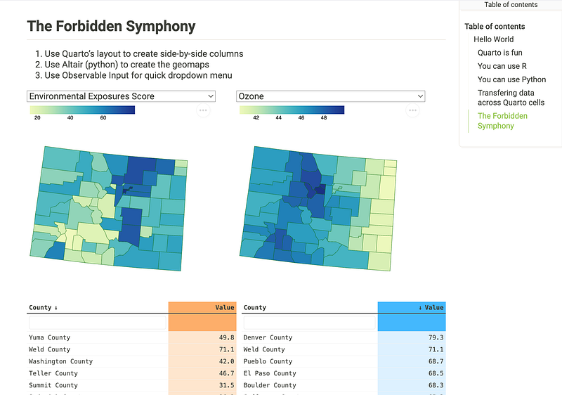
Warning: This is admittedly ugly, to the point of, “Why not just JavaScript?”

What is Quarto?

For those not familiar, Quarto is what I’d describe as publishing tool that turns code-as-deliverable-output (e.g. websites, presentation, papers) toolkit that Posit (formerly R Studio) is spend a lot of time developing into a robust reporting solution, particularly with the focus of handling most cases (actual paper publishing to regulatory grade reports) in the science and life sciences industry.

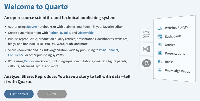
How Quarto achieves this

Markdown enhancement by using their own .qmd file format. Markdown is most often used in Git repository codebase as the README.md, and most people just stop at that. It’s as if the world thinks Markdown only exists for README.md.

There are plenty of flavors of Markdown. I’ve personally used flavors of restructred Markdown (.rst), R Markdown (.Rmd), Markedly Structured Text (.md but with special commands) and whenever your favorite editors have Markdown support, I get curious about the extensions/styling and try it out. (Tidbit: Did you know ChatGPT tries to encourage prompt answers to be in Markdown?)

How I’ve been using Quarto: A Standalone, fully-embedded HTML Generator

I’ve grown really sick of unnecessarily complex data pipelines in “modern data stack” analytics, when most of us need reports, not interactive dashboards.

Why do we need to start thinking about:

SQL servers (when we have DuckDB)

BI tool

Data governance

Cloud IAM / Permissions management

… And so on

I just want some insights from a CSV/Parquet file that I can narrow down to <100k rows? I can assure you that it’ll be data checked. Particularly for datasets that needs “discovery analytics”, shouldn’t we find good analysis first and THEN develop the above checkpoints as business demand increases?

I feel that we don’t do this enough — prototyping to make sure the insights are there. Don’t create a process to that may slow down time-sensitive analytics.

How I’ve been using Quarto: A Standalone, fully-embedded HTML Generator

I won’t go into getting started with Quarto, but I have installed:

Step 1: Create .qmd scaffolding for HTML generation

It took me hours of experimenting to come up with some of these headers in Quarto, to generate embedded HTML.

To brush up on your Markdown, lets create your first medium_tutorial_1.qmd

---
title: "Hello Quarto"
subtitle: "Standalone HTML"
date: "2023-02-22"
author: Jung Hoon Son
title-block-banner: '#F8F5F0'
title-block-banner-color: '#325D88'
toc: true
toc-expand: true
format:
    html:
        theme: sandstone
        embed-resources: true
        font-color: '#325D88'
        linestretch: 1.2
---

# Hello World

## Quarto is fun

## You can use R

## You can use Python

## You can use Observable

Step 2: Preview / Create HTML

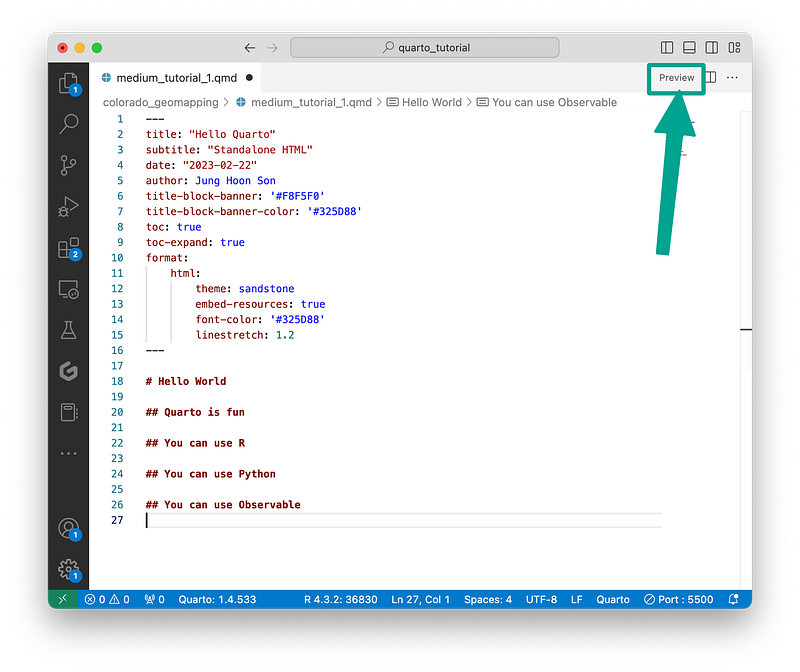
In VS Code, installing the Quarto VS Code extension will give you support for “Preview” button with any .qmd files. Click on it.

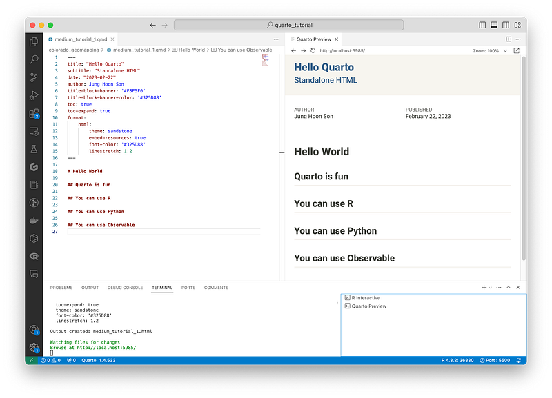
Notice “Output created” with your filename

This by default launches a side-panel preview of the rendered HTML.

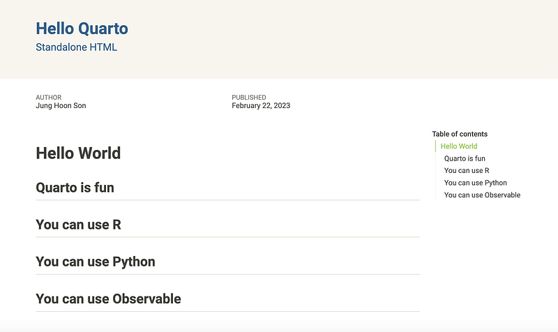
Step 3: Check your Preview and HTML

Try opening your medium_tutorial_1.html located in the same directory as medium_tutorial_1.qmd just to make sure it’s not a VS Code localhost webserver magic.

Step 4: Let’s Add Python code!

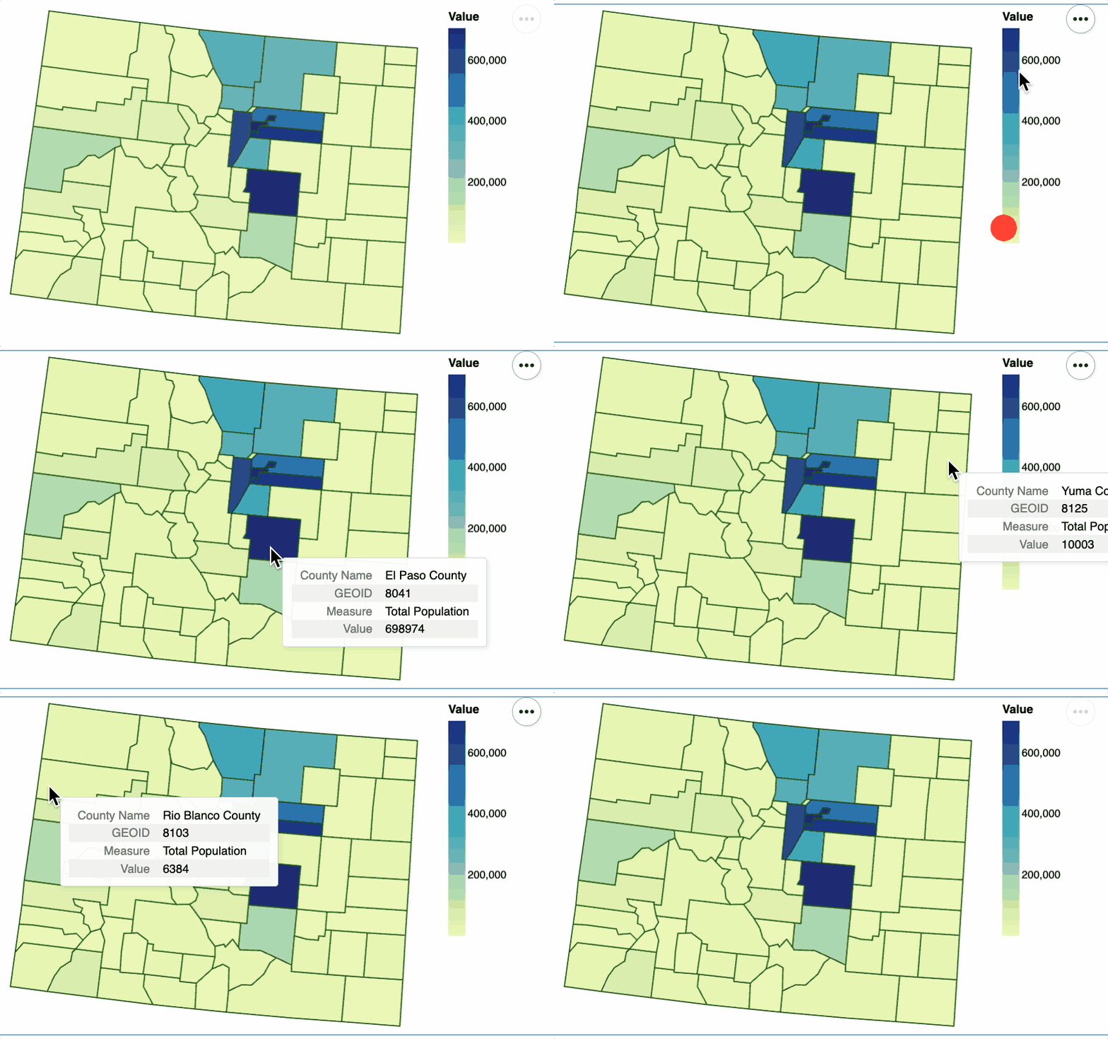
I worked on a geomapping project previously for a “Using Altair to Build a Dynamic, Interactive Choropleth Map” for Altair rendering. Let’s use the same code here.

We will try to recreate this, but better with tables.

Step 5: Hold your horses (R and Python together) venv nightmare.

After a lot of experimentation, I came to realize — Quarto is natively an R-based system. That means it runs in an R environment (usually looks for system install of R).

There is no good “virtual environment” for R.

The bottom lineof this… is that when quarto preview command-line is executed, the python it’s looking for system python interpreter for my python code blocks.

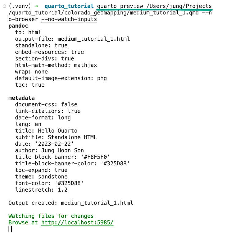
After searching for a bit, I decided to try to explicitly point to which python virtual environment to use… by using reticulate R package, which allows you to point to which virtual environment you’d like to use.

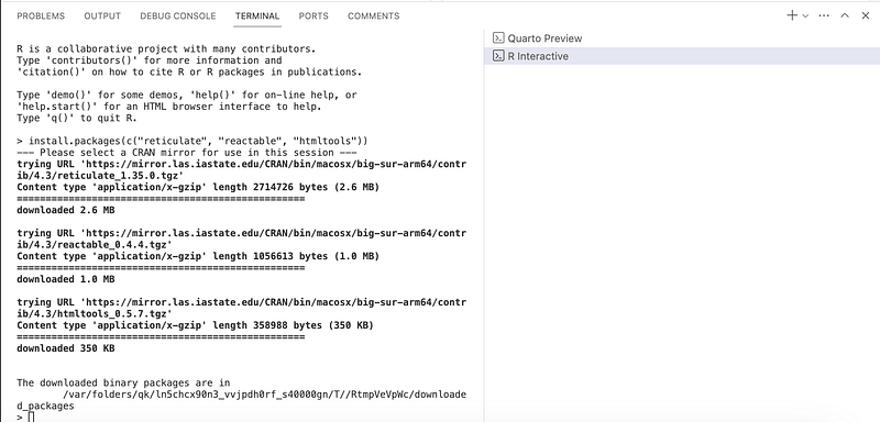
If you haven’t installed R for VS Code and reticulate : here’s a screenshot to explain the craziness that’s about to start.

Installing R packages for this tutorial — reticulate, reactable, htmltools

Step 6: Pointing to Python Virtual Environment from… R code block

My python virtual environment for this project is /Users/jung/Projects/quarto_tutorial/.venv/

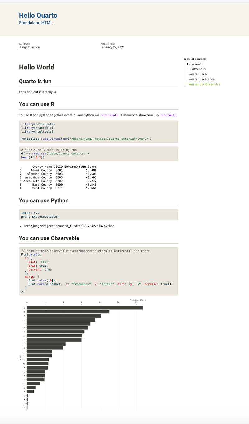
Using reticulate, we can confirm which interpreter it’s using. And let’s showcase that it can actually render all R, Python, Observable codeblocks. Note the codeblock designation syntax:

---
title: "Hello Quarto"
subtitle: "Standalone HTML"
date: "2023-02-22"
author: Jung Hoon Son
title-block-banner: '#F8F5F0'
title-block-banner-color: '#325D88'
toc: true
toc-expand: true
format:
    html:
        theme: sandstone
        embed-resources: true
        font-color: '#325D88'
        linestretch: 1.2
---

# Hello World

## Quarto is fun
Let's find out if it really is.

## You can use R
To use R and python together, need to load python via `reticulate` R libaries to showcase R's `reactable`

```{r}
#| message: false
#| warning: false
library(reticulate)
library(reactable)
library(htmltools)

reticulate::use_virtualenv('/Users/jung/Projects/quarto_tutorial/.venv/')

```

```{r}
# Make sure R code is being run
df <- read.csv("data/County_data.csv")
head(df[0:3])
```

## You can use Python
```{python}
import sys
print(sys.executable)
```

## You can use Observable

```{ojs}
// From https://observablehq.com/@observablehq/plot-horizontal-bar-chart
Plot.plot({
  x: {
    axis: "top",
    grid: true,
    percent: true
  },
  marks: [
    Plot.ruleX([0]),
    Plot.barX(alphabet, {x: "frequency", y: "letter", sort: {y: "x", reverse: true}})
  ]
})
```

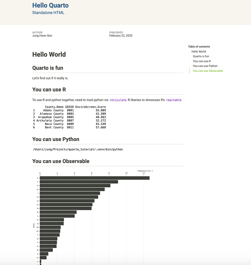
Absolute bonkers rendering of 3 executed code blocks of different languages on HTML

Step 7: Hide the source code

Right under each code block Quarto allows you to enter cell-by-cell configuration.

R:#| echo: false
Python: #| echo: false
Observable: //| echo: false

---
title: "Hello Quarto"
subtitle: "Standalone HTML"
date: "2023-02-22"
author: Jung Hoon Son
title-block-banner: '#F8F5F0'
title-block-banner-color: '#325D88'
toc: true
toc-expand: true
format:
    html:
        theme: sandstone
        embed-resources: true
        font-color: '#325D88'
        linestretch: 1.2
---

# Hello World

## Quarto is fun
Let's find out if it really is.

## You can use R
To use R and python together, need to load python via `reticulate` R libaries to showcase R's `reactable`

```{r}
#| message: false
#| warning: false
#| echo: false
library(reticulate)
library(reactable)
library(htmltools)

reticulate::use_virtualenv('/Users/jung/Projects/quarto_tutorial/.venv/')

```

```{r}
#| echo: false
# Make sure R code is being run
df <- read.csv("data/County_data.csv")
head(df[0:3])
```

## You can use Python
```{python}
#| echo: false
import sys
print(sys.executable)
```

## You can use Observable
Note Observable code isn't fully standalone

```{ojs}
//| echo: false

// From https://observablehq.com/@observablehq/plot-horizontal-bar-chart
Plot.plot({
  x: {
    axis: "top",
    grid: true,
    percent: true
  },
  marks: [
    Plot.ruleX([0]),
    Plot.barX(alphabet, {x: "frequency", y: "letter", sort: {y: "x", reverse: true}})
  ]
})
```

The (not-so) Forbidden Symphony: Quarto, Observable, Python, and R

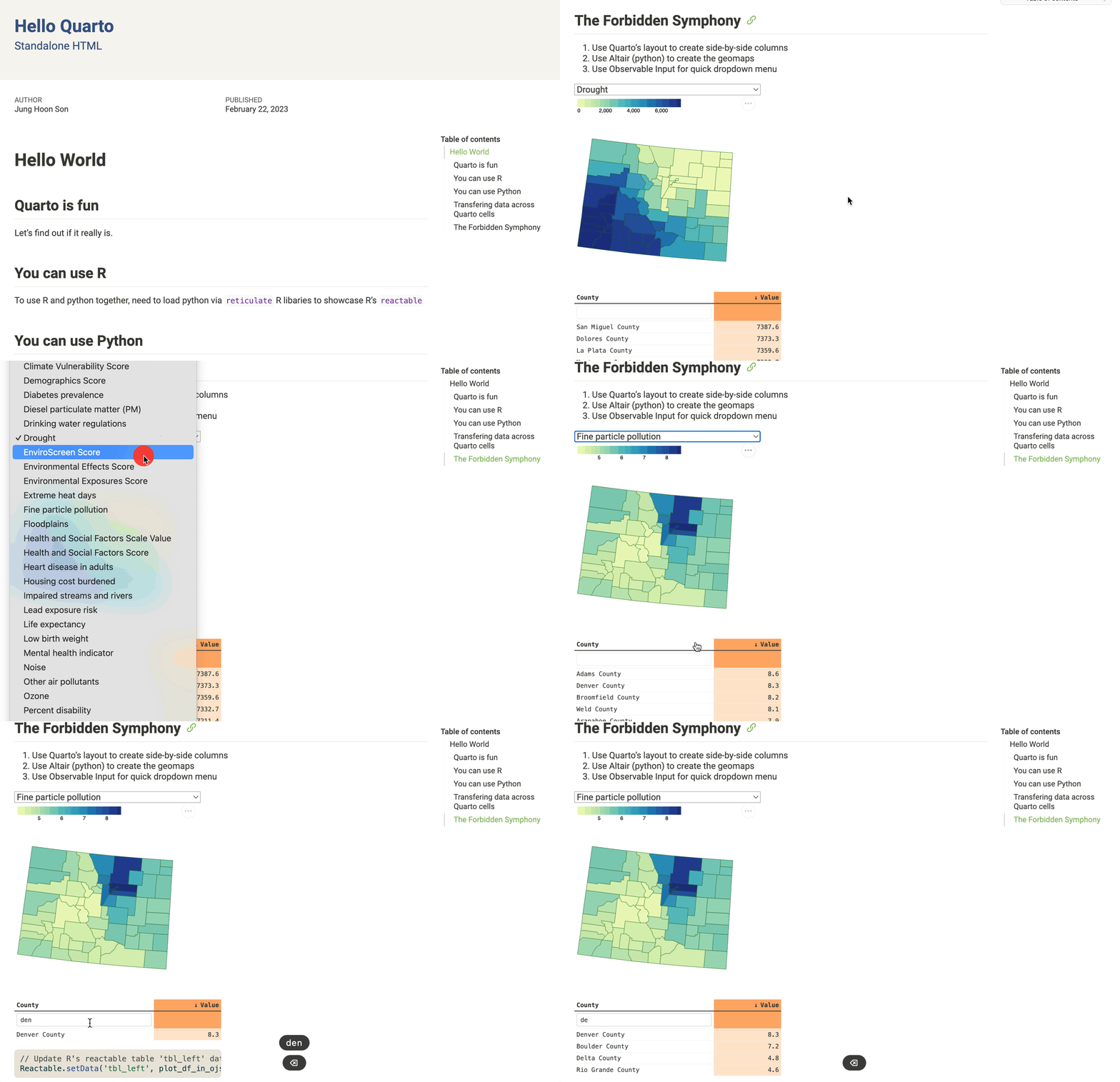
Use Observable drop-down menu to dynamically change the Python’s Altair-generated code

This is admittedly wild, hacky way to make sure the output is good.

Key takeaways for HTML knitting using Quarto:

Observable cannot transfer data back to R/Python
Python cannot transfer data to Observable
R becomes your hub for data “transfers”

Here’s a preview before the code on the bottom

---
title: "Hello Quarto"
subtitle: "Standalone HTML"
date: "2023-02-22"
author: Jung Hoon Son
title-block-banner: '#F8F5F0'
title-block-banner-color: '#325D88'
toc: true
toc-expand: true
format:
    html:
        theme: sandstone
        embed-resources: true
        font-color: '#325D88'
        linestretch: 1.2
---

# Hello World

## Quarto is fun
Let's find out if it really is.

## You can use R
To use R and python together, need to load python via `reticulate` R libaries to showcase R's `reactable`

```{r}
#| message: false
#| warning: false
#| echo: false
library(reticulate)
library(reactable)
library(htmltools)

reticulate::use_virtualenv('/Users/jung/Projects/quarto_tutorial/.venv/')

```


## You can use Python
```{python}
#| message: false
#| warning: false
#| echo: false
#| error: false
import polars as pl
import polars.selectors as cs
import altair as alt
from vega_datasets import data

alt.data_transformers.disable_max_rows()


raw_data = (pl.read_csv("data/County_data.csv", null_values="NA"))
raw_data_pandas = raw_data.select(~cs.contains("Percentile")).to_pandas()

colorado_enviro = (raw_data
    .select(~cs.contains("Percentile"))
    .drop(
        "Prior Disproportionately Impacted Community (January 2023-May 2023)",
        "area", 
        "Justice40", 
        "Disproportionately Impacted Community (May 2023)", 
        "AQCC Reg 3 Disproportionately Impacted Community"
    )
)

colorado_enviro_pandas = colorado_enviro.to_pandas()

plot_df = (
    colorado_enviro.drop("area")
    .melt(id_vars=["County Name", "GEOID"], value_name="value", variable_name="metric")
    .with_columns(
        pl.col("value").cast(pl.Float64),
        pl.when(
            pl.col("metric").str.contains("Percentile"))
            .then(pl.lit("metric_percentile"))
            .otherwise(pl.lit("metric_value")).alias("percentile")
    )
)

counties = alt.topo_feature(data.us_10m.url, "counties")

# Long or "Tidy" dataframes are necessary for plotting
plot_df = (
    colorado_enviro
    .melt(
        id_vars=["County Name", "GEOID"], 
        value_name="value", 
        variable_name="metric")
    .with_columns(
        pl.col("value").cast(pl.Float64)
    )
)

# reticulate only supports pandas df transfer right now
plot_df_pandas = plot_df.fill_null(0).to_pandas()

# Admittedly mark_geoshape() is not the most intuitive function
# `counties`` data is a GeoJSON that contains 
# shapefiles (polygon information for county/state)

# In general GEOID or FIPS codes should generally be 
# considered equivalent, sometimes the GEOID tends to 
# concatenate country/state.
state_zoom = (
    alt.Chart(plot_df)
    .mark_geoshape(strokeWidth=0.5, stroke="darkgreen")
    .encode(
        shape="geo:G",
        color=(
            alt.Color("value:Q")
            .legend(
                orient="top", 
                labelFontSize=10, 
                titleAlign='left')
            .title(None)
        ),
        tooltip=["County Name", "GEOID", "metric", "value"],
    )
    .transform_lookup(
        lookup="GEOID", 
        from_=alt.LookupData(data=counties, key="id"), 
        as_="geo"
    )
    .transform_filter(
        alt.datum.metric=="Total Population"
    )
    .project(type="albersUsa")
    .properties(width=300, height=300)
)

state_zoom_json = state_zoom.to_json()

metrics_list = sorted(plot_df.select("metric").unique().to_series().to_list())

state_zoom

```


## Transfering data across Quarto cells
Quarto does have some functions in development to transfer data across languages

One is via `reticulate` and other is via observable's `ojs_define()`.

Transferring anything from python side transfer is the most problems, and the only way to make python virtual environment currently is to use this workaround of
`python` --> `R` --> `Observable`

Reticulate issues:
- Feature request: Support Polars DataFrames https://github.com/rstudio/reticulate/issues/1319


```{r}
#| column: page
#| echo: false

metrics_list_in_r = py$metrics_list
state_zoom_json_in_r = py$state_zoom_json
plot_df_in_r = py$plot_df_pandas
raw_data_in_r = py$raw_data_pandas
colorado_enviro_in_r = py$colorado_enviro_pandas

ojs_define(metrics_list_in_r)
ojs_define(plot_df_in_r)
ojs_define(colorado_enviro_in_r)
ojs_define(raw_data_in_r)
ojs_define(state_zoom_json_in_r)
```



## The Forbidden Symphony 

1. Use Quarto's layout to create side-by-side columns
2. Use Altair (python) to create the geomaps
3. Use Observable Input for quick dropdown menu


```{ojs}
//| echo: false

import { vl } from "@vega/vega-lite-api"

embed = require("vega-embed@6")

colorado_chloropleth_vl_left = JSON.parse(state_zoom_json_in_r)
colorado_chloropleth_vl_right = JSON.parse(state_zoom_json_in_r)

```


:::: {.columns padding="10px"}

::: {.column width="50%" margin="0.10em"}

```{ojs}
//| echo: false

// Creates an Observable "viewof" for
// 1) dropdown
// 2) choropleth mapping
// `selected_metric` above.

// DROPDOWN: Observable Input dropdown menu, defaults to "Drought"
viewof selected_metric = Inputs.select(metrics_list_in_r, {value: "Drought"})

// CHOROPLETH MAP: Hardcoding the `transform` key to Vega's second array item [1]
// First array items is [0] - the base ID-to-polygon mapping.
// Alternative ideas welcome 
viewof colorado_chloropleth_left = {
    colorado_chloropleth_vl_left.transform[1].filter = `(datum.metric === '${selected_metric}')`
    return embed(colorado_chloropleth_vl_left);
}

// For the Observable cell to register the data we use transpose() to retrieve
// any compatible objects from R
plot_df_in_ojs = transpose(plot_df_in_r)

// FILTERING DATA: Observable/Javascript way to just returning the 
// cells that match "metric" columns == "Drought", think there are better ways
plot_df_in_ojs_filtered = plot_df_in_ojs.filter(data_row => {
  return data_row.metric.includes(selected_metric)
})
```


```{r}
#| message: false
#| warning: false
#| echo: false
#| error: false

# library(htmltools)

reactable_table <- (
    reactable(
        plot_df_in_r,
        elementId = "tbl_left",
        # searchable = TRUE,
        defaultPageSize = 100,
        defaultSorted = c("value"),
        defaultSortOrder = "desc",
        theme = reactableTheme(
            headerStyle = list(
                "&:hover[aria-sort]" = list(background = "#F5F4F3"),
                "$aria-sort='ascending'], &[aria-sort='descending']" = list(background="#F4F3F3"),
                borderColor = "#555"
            ),
            cellPadding = "4px",
        ),
        style=list(
            fontFamily = "monospace",
            fontSize = "0.7rem",
            paddingTop = "1px",
            paddingBottom = "1px"
        ),
        columns = list(
            metric = colDef(
                show=FALSE,
                name="Metric",
                minWidth=100
            ),
            "County Name" = colDef(
                name="County",
                filterable = TRUE,
                # headerStyle = list(background="#fdae6b"),
                minWidth=100
            ),
            GEOID = colDef(show=FALSE),
            value = colDef(
                name="Value",
                maxWidth=130,
                format = colFormat(digits = 1),
                style = list(background="#fee6ce"),
                headerStyle=list(background="#fdae6b"),
            )
        )
    )
)
reactable_table
```


```{ojs}
// Update R's reactable table 'tbl_left' data when filtered data changes
Reactable.setData('tbl_left', plot_df_in_ojs_filtered)
```

:::

::::

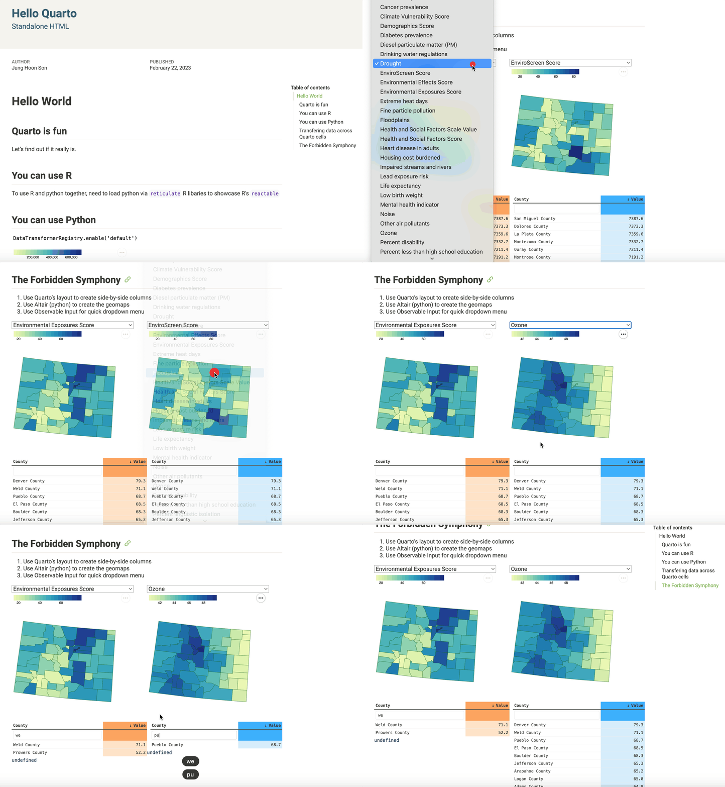
Lastly, side-by-side comparison, be repeating the element above to a new Quarto layout “column” I created using ::: notation.

Entire code:

---
title: "Hello Quarto"
subtitle: "Standalone HTML"
date: "2023-02-22"
author: Jung Hoon Son
title-block-banner: '#F8F5F0'
title-block-banner-color: '#325D88'
toc: true
toc-expand: true
format:
    html:
        theme: sandstone
        embed-resources: true
        font-color: '#325D88'
        linestretch: 1.2
---

# Hello World

## Quarto is fun
Let's find out if it really is.

## You can use R
To use R and python together, need to load python via `reticulate` R libaries to showcase R's `reactable`

```{r}
#| message: false
#| warning: false
#| echo: false
library(reticulate)
library(reactable)
library(htmltools)

reticulate::use_virtualenv('/Users/jung/Projects/quarto_tutorial/.venv/')

```


## You can use Python
```{python}
#| message: false
#| warning: false
#| echo: false
#| error: false
import polars as pl
import polars.selectors as cs
import altair as alt
from vega_datasets import data

alt.data_transformers.disable_max_rows()


raw_data = (pl.read_csv("data/County_data.csv", null_values="NA"))
raw_data_pandas = raw_data.select(~cs.contains("Percentile")).to_pandas()

colorado_enviro = (raw_data
    .select(~cs.contains("Percentile"))
    .drop(
        "Prior Disproportionately Impacted Community (January 2023-May 2023)",
        "area", 
        "Justice40", 
        "Disproportionately Impacted Community (May 2023)", 
        "AQCC Reg 3 Disproportionately Impacted Community"
    )
)

colorado_enviro_pandas = colorado_enviro.to_pandas()

plot_df = (
    colorado_enviro.drop("area")
    .melt(id_vars=["County Name", "GEOID"], value_name="value", variable_name="metric")
    .with_columns(
        pl.col("value").cast(pl.Float64),
        pl.when(
            pl.col("metric").str.contains("Percentile"))
            .then(pl.lit("metric_percentile"))
            .otherwise(pl.lit("metric_value")).alias("percentile")
    )
)

counties = alt.topo_feature(data.us_10m.url, "counties")

# Long or "Tidy" dataframes are necessary for plotting
plot_df = (
    colorado_enviro
    .melt(
        id_vars=["County Name", "GEOID"], 
        value_name="value", 
        variable_name="metric")
    .with_columns(
        pl.col("value").cast(pl.Float64)
    )
)

# reticulate only supports pandas df transfer right now
plot_df_pandas = plot_df.fill_null(0).to_pandas()

# Admittedly mark_geoshape() is not the most intuitive function
# `counties`` data is a GeoJSON that contains 
# shapefiles (polygon information for county/state)

# In general GEOID or FIPS codes should generally be 
# considered equivalent, sometimes the GEOID tends to 
# concatenate country/state.
state_zoom = (
    alt.Chart(plot_df)
    .mark_geoshape(strokeWidth=0.5, stroke="darkgreen")
    .encode(
        shape="geo:G",
        color=(
            alt.Color("value:Q")
            .legend(
                orient="top", 
                labelFontSize=10, 
                titleAlign='left')
            .title(None)
        ),
        tooltip=["County Name", "GEOID", "metric", "value"],
    )
    .transform_lookup(
        lookup="GEOID", 
        from_=alt.LookupData(data=counties, key="id"), 
        as_="geo"
    )
    .transform_filter(
        alt.datum.metric=="Total Population"
    )
    .project(type="albersUsa")
    .properties(width=300, height=300)
)

state_zoom_json = state_zoom.to_json()

metrics_list = sorted(plot_df.select("metric").unique().to_series().to_list())

state_zoom

```


## Transfering data across Quarto cells
Quarto does have some functions in development to transfer data across languages

One is via `reticulate` and other is via observable's `ojs_define()`.

Transferring anything from python side transfer is the most problems, and the only way to make python virtual environment currently is to use this workaround of
`python` --> `R` --> `Observable`

Reticulate issues:
- Feature request: Support Polars DataFrames https://github.com/rstudio/reticulate/issues/1319


```{r}
#| column: page
#| echo: false

metrics_list_in_r = py$metrics_list
state_zoom_json_in_r = py$state_zoom_json
plot_df_in_r = py$plot_df_pandas
raw_data_in_r = py$raw_data_pandas
colorado_enviro_in_r = py$colorado_enviro_pandas

ojs_define(metrics_list_in_r)
ojs_define(plot_df_in_r)
ojs_define(colorado_enviro_in_r)
ojs_define(raw_data_in_r)
ojs_define(state_zoom_json_in_r)
```



## The Forbidden Symphony 

1. Use Quarto's layout to create side-by-side columns
2. Use Altair (python) to create the geomaps
3. Use Observable Input for quick dropdown menu


```{ojs}
//| echo: false

import { vl } from "@vega/vega-lite-api"

embed = require("vega-embed@6")

colorado_chloropleth_vl_left = JSON.parse(state_zoom_json_in_r)
colorado_chloropleth_vl_right = JSON.parse(state_zoom_json_in_r)

```


:::: {.columns padding="10px"}

::: {.column width="50%" margin="0.10em"}

```{ojs}
//| echo: false

// Creates an Observable "viewof" for
// 1) dropdown
// 2) choropleth mapping
// `selected_metric` above.

// DROPDOWN: Observable Input dropdown menu, defaults to "Drought"
viewof selected_metric = Inputs.select(metrics_list_in_r, {value: "Drought"})

// CHOROPLETH MAP: Hardcoding the `transform` key to Vega's second array item [1]
// First array items is [0] - the base ID-to-polygon mapping.
// Alternative ideas welcome 
viewof colorado_chloropleth_left = {
    colorado_chloropleth_vl_left.transform[1].filter = `(datum.metric === '${selected_metric}')`
    return embed(colorado_chloropleth_vl_left);
}

// For the Observable cell to register the data we use transpose() to retrieve
// any compatible objects from R
plot_df_in_ojs_right = transpose(plot_df_in_r)

// FILTERING DATA: Observable/Javascript way to just returning the 
// cells that match "metric" columns == "Drought", think there are better ways
plot_df_in_ojs_filtered = plot_df_in_ojs_right.filter(data_row => {
  return data_row.metric.includes(selected_metric)
})
```


```{r}
#| message: false
#| warning: false
#| echo: false
#| error: false

# library(htmltools)

reactable_table <- (
    reactable(
        plot_df_in_r,
        elementId = "tbl_left",
        # searchable = TRUE,
        defaultPageSize = 100,
        defaultSorted = c("value"),
        defaultSortOrder = "desc",
        theme = reactableTheme(
            headerStyle = list(
                "&:hover[aria-sort]" = list(background = "#F5F4F3"),
                "$aria-sort='ascending'], &[aria-sort='descending']" = list(background="#F4F3F3"),
                borderColor = "#555"
            ),
            cellPadding = "4px",
        ),
        style=list(
            fontFamily = "monospace",
            fontSize = "0.7rem",
            paddingTop = "1px",
            paddingBottom = "1px"
        ),
        columns = list(
            metric = colDef(
                show=FALSE,
                name="Metric",
                minWidth=100
            ),
            "County Name" = colDef(
                name="County",
                filterable = TRUE,
                # headerStyle = list(background="#fdae6b"),
                minWidth=100
            ),
            GEOID = colDef(show=FALSE),
            value = colDef(
                name="Value",
                maxWidth=130,
                format = colFormat(digits = 1),
                style = list(background="#fee6ce"),
                headerStyle=list(background="#fdae6b"),
            )
        )
    )
)
reactable_table
```


```{ojs}
//| message: false
//| warning: false
//| echo: false
//| error: false

// Update R's reactable table 'tbl_left' data when filtered data changes
Reactable.setData('tbl_left', plot_df_in_ojs_filtered)

```

:::

::: {.column width="50%" margin="0.10em"}

```{ojs}
//| echo: false

// Creates an Observable "viewof" for
// 1) dropdown
// 2) choropleth mapping
// `selected_metric` above.

// DROPDOWN: Observable Input dropdown menu, defaults to "Drought"
viewof selected_metric_right = Inputs.select(metrics_list_in_r, {value: "EnviroScreen Score"})

// CHOROPLETH MAP: Hardcoding the `transform` key to Vega's second array item [1]
// First array items is [0] - the base ID-to-polygon mapping.
// Alternative ideas welcome 
viewof colorado_chloropleth_right = {
    colorado_chloropleth_vl_right.transform[1].filter = `(datum.metric === '${selected_metric_right}')`
    return embed(colorado_chloropleth_vl_right);
}

// For the Observable cell to register the data we use transpose() to retrieve
// any compatible objects from R
plot_df_in_ojs = transpose(plot_df_in_r)

// FILTERING DATA: Observable/Javascript way to just returning the 
// cells that match "metric" columns == "Drought", think there are better ways
plot_df_in_ojs_filtered_right = plot_df_in_ojs.filter(data_row => {
  return data_row.metric.includes(selected_metric_right)
})
```


```{r}
#| echo: false

library(htmltools)

# Conditional formatting in orange
# orange_pal <- function(x) rgb(colorRamp(c("#ffe4cc", "#ffb54d"))(x), maxColorValue = 255)

reactable_table <- (
    reactable(
        plot_df_in_r,
        elementId = "tbl_right",
        # searchable = TRUE,
        defaultPageSize = 100,
        defaultSorted = c("value"),
        defaultSortOrder = "desc",
        defaultExpanded = TRUE,
        # groupBy = c("metric"),
        theme = reactableTheme(
            headerStyle = list(
                "&:hover[aria-sort]" = list(background = "#F5F4F3"),
                "$aria-sort='ascending'], &[aria-sort='descending']" = list(background="#F4F3F3"),
                borderColor = "#555"
            ),
            cellPadding = "4px",
        ),
        style=list(
            fontFamily = "monospace",
            fontSize = "0.7rem",
            marginLeft = "10px",
            paddingTop = "1px",
            paddingBottom = "1px"
        ),
        columns = list(
            metric = colDef(
                show=FALSE,
                name="Metric",
                minWidth=100
            ),
            "County Name" = colDef(
                name="County",
                filterable = TRUE,
                minWidth=100
            ),
            GEOID = colDef(show=FALSE),
            value = colDef(
                name="Value",
                maxWidth=130,
                format = colFormat(digits = 1),
                headerStyle=list(background="#45b8ff"),
                style=list(background="#ddf2ff"),
            )
        )
    )
)
reactable_table
```


```{ojs}
//| message: false
//| warning: false
//| echo: false
//| error: false

// Update R's reactable table 'tbl_left' data when filtered data changes
Reactable.setData('tbl_right', plot_df_in_ojs_filtered)

```

:::

::::

Final Words

In terms of practicality, probably gets to the point of too much complexity in dealing with transferring and keeping track of variables across R/Python/Observable.

Also data is embedded in HTML — exposed.

If you have sensitive data, don’t use this route.

There are some developing features related to Quarto that will probably allow more seamless integration and data/object “transfers”.

I think the biggest takeaway from this exercise is understanding the current direction of the variable transfers and functions.
ojs_define() currently seems to be geared for R Shiny applications and not HTML knitting, which explains some confusion (https://github.com/quarto-dev/quarto-cli/issues/3018).
reticulate need reveals some mechanism to do “multi-virtual-env management” which sounds insane given R and Python suffer from “work in progress” venv issues.

All-in-all, I do feel like I’ve gotten the HTML file I can host. They say backend is always uglier than front end, and front-end output seems clean enough to justify all the work.

Hope you enjoyed this!

-Jung