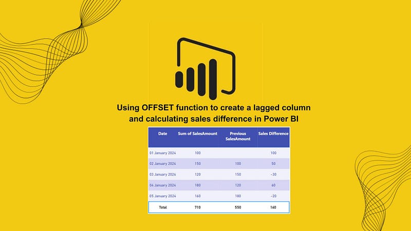
Using OFFSET function to create a lagged column and calculating sales difference in Power BI

In the dynamic world of business analytics, keeping track of sales trends and making informed decisions is paramount. Power BI, a powerful tool from Microsoft, offers a plethora of functionalities to help analysts and business professionals visualize and interpret data efficiently.

One such valuable feature is the use of the OFFSET function to create lagged columns and calculate sales differences over time.

Here’s a quick overview of what we’ll cover in this article:

Understanding the OFFSET Function:

• What is the OFFSET function?
• How it helps in creating lagged columns.
• Practical applications in business analytics.

Creating a Lagged Column in Power BI:

• Step-by-step guide to implementing the OFFSET function.
• Example scenarios to illustrate its utility.

Calculating Sales Difference:

• Methods to compare sales figures over different time periods.
• Using DAX expressions to achieve accurate sales calculations.

Benefits of Using Lagged Columns:

• Enhanced trend analysis.
• Improved forecasting capabilities.
• Identifying patterns and anomalies in sales data.

By the end of this article, you’ll have a solid understanding of how to utilize the OFFSET function in Power BI to enhance your data analysis, making it easier to track sales trends and make strategic decisions.

Implementation in Power BI:

Here are all the steps we will be following in the step-by-step guide to help you set it up:

• Grasping the Table Structure
• Writing the DAX function for lagged SalesAmount column
• Obtaining the sales difference between current and previous day

Happy learning!

1.Grasping the Table Structure:

Before diving into the functionalities of the OFFSET function, it’s crucial to have a clear understanding of the table we’ll be working with.

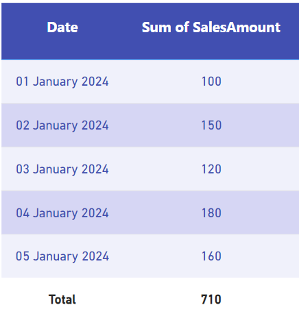
The table is named SalesTable.

Table Overview

This table records sales data over a period of five consecutive days in January 2024. It has two columns:

1. Date: Represents each day from January 1, 2024, to January 5, 2024.
2. SalesAmount: Indicates the amount of sales made on each respective day.

Data Description

• 2024–01–01: Sales amount is 100.
• 2024–01–02: Sales amount increased to 150.
• 2024–01–03: Sales amount decreased to 120.
• 2024–01–04: Sales amount went up significantly to 180.
• 2024–01–05: Sales amount slightly decreased to 160.

This data is useful for analyzing sales trends over the specified period, helping to understand the daily fluctuations and overall sales performance.

2. Writing the DAX function for lagged SalesAmount column:

Now we will be using the OFFSET function to lag the SalesAmount column by one day one the basis of Date column.

Previous SalesAmount = CALCULATE(SUM(‘SalesTable’[SalesAmount]), OFFSET(-1, ALLSELECTED(‘SalesTable’[Date]), ORDERBY(‘SalesTable’[Date], ASC)))

Explanation:

1. CALCULATE: This function modifies the context in which data is evaluated.

• It evaluates the SUM('SalesTable'[SalesAmount]) within the given context.

2. SUM(‘SalesTable’[SalesAmount]):

• This part of the formula sums up the SalesAmount column from the 'SalesTable' table.

3. OFFSET:

• -1: This indicates that we want to move one row up (previous row) or the number of rows before (negative value) the current row from which to obtain the data.
• ALLSELECTED(‘SalesTable’[Date]): This argument defines the base set of data for the operation, taking all selected dates into account.
• ORDERBY(‘OSalesTable’[Date], ASC): This orders the rows by the Date column in ascending order.

Purpose:

This DAX formula is designed to calculate the SalesAmount for the previous date relative to each row in the 'SalesTable' table. Here's a step-by-step rundown of how it works:

• ALLSELECTED('SalesTable'[Date]) establishes the base data set by including all selected dates.
• ORDERBY('SalesTable'[Date], ASC) sorts these dates in ascending order.
• OFFSET(-1, ...) shifts the context by one row up (previous date) or the number of rows before (negative value) the current row from which to obtain the data.
• SUM('SalesTable'[SalesAmount]) then sums the SalesAmount for the previous date.
• CALCULATE(...) evaluates the sum in the modified context created by the OFFSET function.

This formula is useful for creating a lagged column where each row displays the sales amount of the previous day, allowing for further analysis, such as calculating the difference in sales between consecutive days.

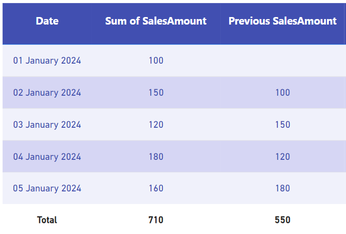
Since we don’t have any data for the dates before 2024–01–01, Previous SalesAmount takes blank value in the first cell and for all the other rows the it takes the value of the previous date.

3. Obtaining the sales difference between current and previous day:

Next we will use a simple DAX to find the difference between SalesAmount and Previous SalesAmount for each day.

Sales Difference = SUM(‘SalesTable’[SalesAmount]) — [Previous SalesAmount]

Explanation:

• SUM(‘SalesTable’[SalesAmount]): Retrieves the current row’s SalesAmount.
• [Previous SalesAmount]: Refers to the previously calculated sales amount from the prior date.
• Sales Difference: Calculates the difference between the current row’s sales and the previous day’s sales.

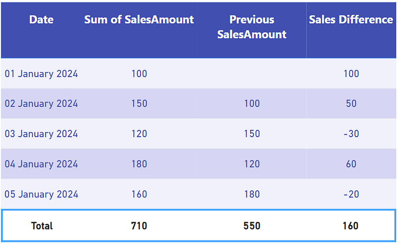
Given the table with Date, SalesAmount, and Previous SalesAmount, the Sales Difference measure computes the daily change in sales, helping you understand how sales are evolving over time.

And with we have successfully used the OFFSET function to first find the Sales amount for previous day and then the sales difference between the current and previous day.

The same thing has been historically being done in SQl and Spreadsheets and now we can very easily do it on Microsoft Power BI too.

Download the data for the above from this link.

Thank you for your attention!

Follow me or subscribe to get all my Power BI articles!

Don’t forget to subscribe to

👉 Power BI Publication

👉 Power BI Newsletter

and join our Power BI community: