Using Forward-search algorithms to solve AI Planning Problems

Let’s use deterministic version of forward-search algorithms to solve AI Planning Problems

If you haven’t read previous post about data representation, to get more context, you can read that post first.

Forward-search

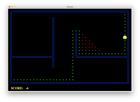
Forward-search is a technique to find a solution to a Planning Problem by searching forward from the initial state to find a sequence of actions that reaches the goal (desired) states.

There are many algorithms that fall into this category.

In this post, we’ll discuss about domain-independent algorithms as opposed to domain-specific algorithms such as path or motion planning domain. Though most if not all of them can be applied to path or motion planning as well.

The following is the pseudo code of forward-search algorithm.

# pp is short for planning_problem
Forward-search(pp):
 current_state = pp.initial_state
 plan = []
 while True:
  if current_state == pp.goal_state:
   return plan
  applicable_actions = pp.get_applicable_actions(current state)
  if not applicable_actions:
    return None  # failure
  action = choose_action(applicable_actions)
  current_state = pp.predict_state(current_state, action)
  plan.append(action)

The algorithm get applicable actions, choose one of them, predict the resultant state and continue iteratively until it finds either the goal state or a no more applicable actions which means that the algorithm has failed to find a solution.

Deterministic-search

In this post we specifically look into deterministic version of forward-search, based on “Automated Planning and Acting” book.

Here is the generic version of the algorithm which can be derived by many variety of forward-search algorithms which we will see later.

We focus on search function to understand how this algorithm works.

Before we look into the algorithm, first we understand a few concepts.

Frontier is the list of nodes that are ready to be visited whereas Expanded is the list of nodes that has been visited so far.

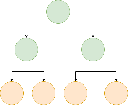
If we illustrate the nodes in tree like in the picture above, those nodes in green are visited nodes and those nodes in orange are frontier (candidates to be visited) nodes.

Starting the algorithm

We start the algorithm by adding initial state or root node to Frontier list before we execute the algorithm.

Executing the algorithm

These are the main steps in the algorithm.

1. Select a node from Frontier This is an important step and is implemented differently by different algorithms
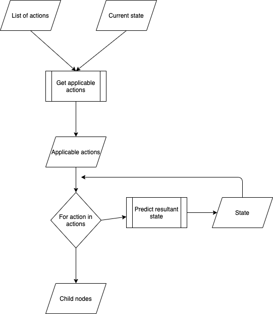
2. If the selected node is not the goal, the child nodes are generated This is the process where we use Action Templates to search for applicable actions in current state. We then predict the resultant states by applying the actions to current state (see picture below).
3. This step is to construct the node by adding successor, predecessor and the total cost of actions so far
4. We then compute the heuristic value This step is basically helping the algorithm to not explore the entire search space because it can be exponentially large, which will make the algorithm runs slowly
5. Prune the nodes This too is a step implemented differently by different algorithms to remove unpromising nodes. One common thing in this step is to do cycle-checking to ensure that an algorithm terminates, not entering infinite loop. In some algorithms this step removes nodes from Child Nodes which is not following current direction. We’ll see more when we discuss instances of this generic algorithm.

Ending the algorithm

The algorithm continues to run until it finds a solution (goal state) or has empty Frontier which means it has failed to find a solution to the Planning Problem.

Heuristic Function

In step 4 we compute a heuristic which is an informed guess to help the algorithm move towards parts of the search space that are likely to lead to solutions.

h(s)≈h*(s)=min⁡{cost(π)∣γ(s,π) satisfies g}

We choose the likely lowest cost for all paths such that predicted resultant state satisfy goal state.

In the next post we’ll look into instances of this algorithm and the examples in solving problems. They are:

• Breadth-first search (BFS)
• Depth-first search (DFS)
• Hill-climbing (Greedy)
• Uniform-cost search
• A*
• Greedy Best-first search (GBFS)
• DFS Branch and Bound