Unraveling the Design Pattern of Physics-Informed Neural Networks: Part 06

Bring causality to PINN training

Welcome to the 6th blog of this series, where we continue our exciting journey of exploring design patterns of physics-informed neural networks (PINN)🙌

In this episode, we will talk about bringing causality to the training of physics-informed neural nets. As suggested by the paper we will look at today: respecting causality is all you need!

As always, let’s begin by talking about the current matters in question, then move on to the suggested remedies, the evaluation procedure, and the advantages and disadvantages of the proposed method. Finally, we will conclude the blog by exploring potential opportunities that lie ahead.

As this series continues to expand, the collection of PINN design patterns grows even richer🙌 Here’s a sneak peek at what awaits you:

PINN design pattern 01: Optimizing the residual point distribution

PINN design pattern 02: Dynamic solution interval expansion

PINN design pattern 03: Training PINN with gradient boosting

PINN design pattern 04: Gradient-enhanced PINN learning

PINN design pattern 05: Automated hyperparameter tuning

PINN design pattern 07: Active learning with PINN

Let’s dive in!

1. Paper at a glance 🔍

• Title: Respecting causality is all you need for training physics-informed neural networks
• Authors: S. Wang, S. Sankaran, P. Perdikaris
• Institutes: University of Pennsylvania
• Link: arXiv, GitHub

2. Design pattern 🎨

2.1 Problem 🎯

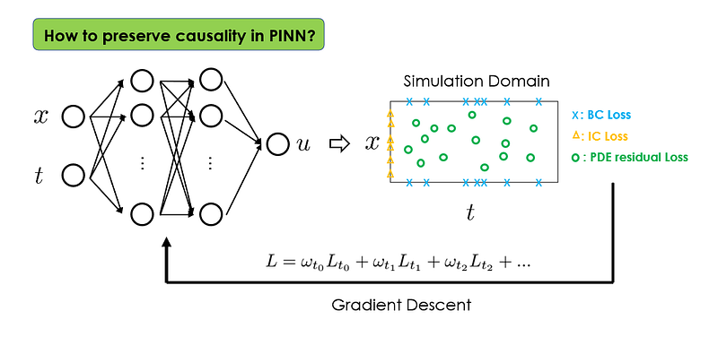
Physics-informed neural networks (PINNs) are a major leap in combining observational data and physical laws across various fields. In practice, however, they are often observed to be unable to tackle high nonlinearity, multi-scale dynamics, or chaotic problems, and tend to converge to erroneous solutions.

Why this is the case?

Well, the fundamental issue lies in the violation of causality in the PINN formulations, as revealed by the current paper.

Causality, in the physical sense, implies that the state at a future time point depends on the state at the current or past time points. In PINN training, however, this principle may not hold true; these networks might be implicitly biased towards first approximating PDE solutions at future states before even resolving initial conditions, essentially “jumping ahead” in time and thereby violating causality.

In contrast, traditional numerical methods inherently preserve causality via a time-marching strategy. For instance, when discretizing PDE in time, these methods ensure the solution at time t is resolved before approximating the solution at time t + ∆t. Hence, each future state is sequentially built upon the resolved past states, thus preserving the principle of causality.

This understanding of the problem brings us to an intriguing question: how do we rectify this violation of causality in PINNs, bringing them in line with fundamental physical laws?

2.2 Solution 💡

The key idea here is to re-formulate the PINN loss function.

Specifically, we can introduce a dynamic weighting scheme to account for different contributions of PDE residual loss evaluated at different temporal locations. Let’s break it down using illustrations.

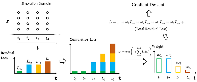
For simplicity, let’s assume the collocation points are uniformly sampled in the spatial-temporal domain of our simulation, as illustrated in the figure below:

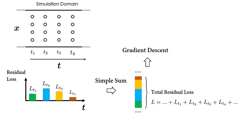
To proceed with one step of gradient descent, we must first calculate the cumulative PDE residual loss across all collocation points. One specific way to do that is by first calculating the losses related to the collocation points sampled at individual time instances, and then performing a “simple sum” to get the total loss. The following gradient descent step can then be conducted based on the calculated total loss to optimize the PINN weights.

Of course, the exact order of summation over collocation points doesn’t influence the total loss computation; all methods yield the same result. However, the decision to group loss calculations by temporal order is purposeful, designed to emphasize the element of ‘temporality’. This concept is crucial for understanding the proposed causal training strategy.

In this process, the PDE residual losses evaluated at different temporal locations are treated equally. meaning that all temporal residual losses are simultaneously minimized.

This approach, however, risks the PINN violating temporal causality, as it doesn’t enforce a chronological regularization for minimizing the temporal residual loss at successive time intervals.

So, how can we coax PINN to adhere to the temporal precedence during training?

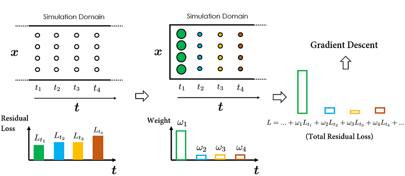
The secret is in selectively weighting individual temporal residual losses. For instance, suppose that at the current iteration, we want the PINN to focus on approximating the solutions at time instance t₁. Then, we could simply put a higher weight on Lᵣ(t₁), which is the temporal residual loss at t₁. This way, Lᵣ(t₁) will become a dominant component in the final total loss, and as a result, the optimization algorithm will prioritize minimizing Lᵣ(t₁), which aligns with our goal of approximating solutions at time instance t₁ first.

In the subsequent iteration, we shift our focus to the solutions at time instance t₂. By increasing the weight on Lᵣ(t₂), it now becomes the main factor in the total loss calculation. The optimization algorithm is thus directed towards minimizing Lᵣ(t₂), improving the prediction accuracy of the solutions at t₂.

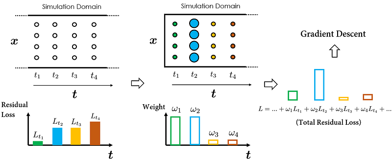
As can be seen from our previous walk-through, varying the weights assigned to temporal residual losses at different time instances enables us to direct the PINN to approximate solutions at our chosen time instances.

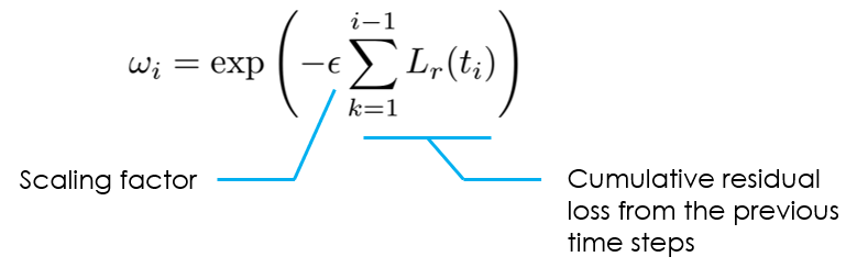
So, how does this assist in incorporating a causal structure into PINN training? It turns out, we can design a causal training algorithm (as proposed in the paper), such that the weight for the temporal residual loss at time t, i.e., Lᵣ(t), is significant only when the losses before t (Lᵣ(t-1), Lᵣ(t-2), etc.) are sufficiently small. This effectively means that the neural network begins minimizing Lᵣ(t) only when it has achieved satisfactory approximation accuracy for prior steps.

To determine the weight, the paper proposed a simple formula: the weight ωᵢ is set to be inversely exponentially proportional to the magnitude of the cumulative temporal residual loss from all the previous time instances. This ensures that the weight ωᵢ will only be active (i.e., with a sufficiently large value) when the cumulative loss from all previous time instances is small, i.e., PINN can already accurately approximate solutions at previous time steps. This is how temporal causality is reflected in the PINN training.

With all components explained, we can piece together the full causal training algorithm as follows:

Before we conclude this section, there are two remarks worth mentioning:

1. The paper suggested using the magnitude of ωᵢ as the stopping criterion for PINN training. Specifically, when all ωᵢ’s are larger than a pre-defined threshold δ, the training may be deemed completed. The recommended value for δ is 0.99.
2. Selecting a proper value for ε is important. Although this value can be tuned via conventional hyperparameter tuning, the paper recommended an annealing strategy for adjusting ε. Details can be found in the original paper (section 3).

2.3 Why the solution might work 🛠️

By dynamically weighting temporal residual losses evaluated at different time instances, the proposed algorithm is able to steer the PINN training to first approximate PDE solutions at earlier times before even trying to resolve the solution at later times.

This property facilitates the explicit incorporation of temporal causality into the PINN training and constitutes the key factor in potentially more accurate simulations of physical systems.

2.4 Benchmark ⏱️

The paper considered a total of 3 different benchmark equations. All problems are forward problems where PINN is used to solve the PDEs.

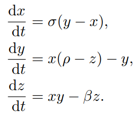
• Lorenz system: these equations arise in studies of convection and instability in planetary atmospheric convection. Lorenz system exhibits strong sensitivity to its initial conditions, and it is known to be challenging for vanilla PINN.

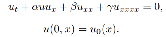
• Kuramoto–Sivashinsky equation: this equation describes the dynamics of various wave-like patterns, such as flames, chemical reactions, and surface waves. It is known to exhibit a wealth of spatiotemporal chaotic behaviors.

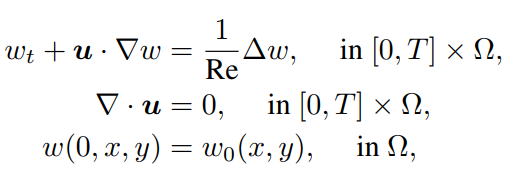
• Navier-Stokes equation: this set of partial differential equations describes the motion of fluid substances and constitutes the fundamental equations in fluid mechanics. The current paper considered a classical two-dimensional decaying turbulence example in a square domain with periodic boundary conditions.

The benchmark studies yielded that:

• The proposed causal training algorithm was able to achieve 10–100x improvements in accuracy compared to the vanilla PINN training scheme.
• Demonstrated that PINNs equipped with causal training algorithm can successfully simulate highly nonlinear, multi-scale, and chaotic systems.

2.5 Strengths and Weaknesses ⚡

Strengths 💪

• Respects the causality principle and makes PINN training more transparent.
• Introduces significant accuracy improvements, allowing it to tackle problems that have remained elusive to PINNs.
• Provides a practical quantitative criterion for assessing the training convergence of PINNs.
• Negligible added computational cost compared to the vanilla PINN training strategy. The only added cost is to compute the ωᵢ’s, which is negligible compared to auto-diff operations.

Weaknesses 📉

• Introduced a new hyperparameter ε, which controls the scheduling of the weights for temporal residual losses. Although the authors proposed an annealing strategy as an alternative to avoid the tedious hyper-parameter tuning.
• Complicated the PINN training workflow. Special attention should be given to the temporal weights ωᵢ’s, as they are now functions of the network trainable parameters (e.g., layer weights and bias), and the gradient associated with the computation of ωᵢ should not be back-propagated.

2.6 Alternatives 🔀

There are a couple of alternative methods that are trying to address the same issue as the current “causal training algorithm”:

• Adaptive time sampling strategy (Wight et al.): instead of weighting the collocation points at different time instances, this strategy modifies the sampling density of collocation points. This has a similar effect of shifting the focus of the optimizer on minimizing temporal losses at different time instances.
• “Time-marching”/“Curriculum training” strategy (e.g., Krishnapriyan et al.): the temporal causality is respected via learning the solution sequentially within separate time windows.

However, compared to those alternative approaches, the “causal training algorithm” put temporal causality front and center, is more adaptable to a variety of problems, and enjoys low added computational cost.

3 Potential Future Improvements 🌟

There are several possibilities to further improve the proposed strategy:

• Incorporating more sophisticated data sampling strategies, such as adaptive- and residual-based sampling methods, to further improve the training efficiency and accuracy.

To learn more about how to optimize the residual points distribution, check out this blog in the PINN design pattern series.

• Extend to inverse problem settings. How to ensure casualty when point sources of information (i.e., observational data) are available would require an extension of the currently proposed training strategy.

4 Takeaways 📝

In this blog, we looked at how to bring causality to PINN training with a reformulation of the training objectives. Here are the highlights of the design pattern proposed in the paper:

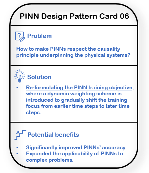
• [Problem]: How to make PINNs respect the causality principle underpinning the physical systems?
• [Solution]: Re-formulating the PINN training objective, where a dynamic weighting scheme is introduced to gradually shift the training focus from earlier time steps to later time steps.
• [Potential benefits]: 1. Significantly improved PINNs’ accuracy. 2. Expanded the applicability of PINNs to complex problems.

Here is the PINN design card to summarize the takeaways:

I hope you found this blog useful! To learn more about PINN design patterns, feel free to check out other posts in this series:

• PINN design pattern 01: Optimizing the residual point distribution
• PINN design pattern 02: Dynamic solution interval expansion
• PINN design pattern 03: PINN training with gradient boost
• PINN design pattern 04: Gradient-enhanced PINN learning
• PINN design pattern 05: Hyperparameter tuning for PINN
• PINN design pattern 07: Active learning with PINN

Looking forward to sharing more insights with you in the upcoming blogs!

Reference 📑

[1] Wang et al., Respecting causality is all you need for training physics-informed neural networks, arXiv, 2022.