Unraveling the Design Pattern of Physics-Informed Neural Networks: Part 03

Supercharging PINN’s performance with gradient boost training

Welcome to the 3rd blog of this series, where we continue our exciting journey of exploring design patterns of physics-informed neural networks (PINN).

In this blog, we will look into training PINNs with gradient boosting, an exciting fusion of neural networks and gradient boosting algorithms 🚀.

As usual, I will structure this blog in the following way:

the problem, the specific problem the proposed strategy is trying to address;
the solution, the key components of the proposed strategy, how it is implemented, and why it might work;
the benchmark, what physical problems are evaluated, and what’s the associated performance;
the strengths & weaknesses, under which conditions the proposed strategy can be effective, while also highlighting its potential limitations;
the alternatives, other approaches proposed to address a similar problem, thus providing a broader perspective on potential solutions.

As this series continues to expand, the collection of PINN design patterns grows even richer🙌 Here’s a sneak peek at what awaits you:

PINN design pattern 01: Optimizing the residual point distribution

PINN design pattern 02: Dynamic solution interval expansion

PINN design pattern 04: gradient-enhanced PINN learning

PINN design pattern 05: automated hyperparameter tuning

PINN design pattern 06: Causal PINN training

PINN design pattern 07: Active learning with PINN

Let’s dive in!

1. Paper at a glance:

Title: Ensemble learning for physics informed neural networks: a Gradient Boosting approach
Authors: Z. Fang, S. Wang, P. Perdikaris
Institutes: University of Pennsylvania
Link: arXiv

2. Design pattern

2.1 Problem

Naive PINNs are known to have difficulties in simulating physical processes that are sensitive to small changes in the input and require a high degree of accuracy to accurately capture their dynamics. Examples of those physical systems include multi-scale problems and singular perturbation problems, which are highly relevant to domains like fluid dynamics and climate modeling.

PINN workflow. Naive PINNs often encounter challenges in solving complicated PDEs. One promising way to address this issue is by training PINNs with **boosting** algorithms. (Image by this blog author)

2.2 Solution

It turns out, the same issue is also experienced by other machine learning algorithms, and a promising way to resolve this issue is by adopting the “Gradient Boosting” method. Therefore, a natural question arises: can we mimic the gradient boosting algorithm to train PINNs? The paper has given a positive answer.

Boosting is a general machine learning algorithm that can be succinctly expressed in the following iterative form:

At each boosting round, an incremental model hₘ(•) is derived and added (discounted by a learning rate ρₘ) on top of the predictor from the last iteration fₘ_₁(•), such that the accuracy of fₘ(•) could be “boosted”.

Now, if we replace fₘ_₁(•), fₘ(•), and hₘ(•) as physics-informed neural networks, we can realize training PINNs with boosting algorithm. A diagram to showcase the training process is given below:

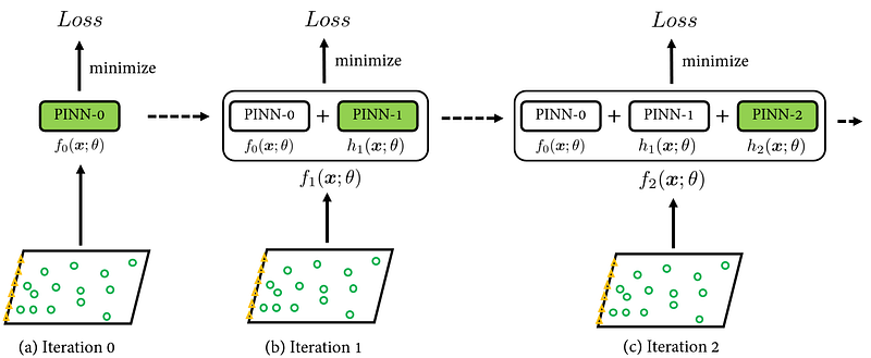
PINN models are trained in sequence to iteratively minimize the loss. Only the blocks marked green are trainable. The loss is the usual PINN loss, i.e., PDE loss, boundary condition loss, etc. (Image by this blog author)

In the paper’s implementation, the architecture and the hyperparameters of the additive PINN model hₘ(•) are pre-determined. This is different from the original gradient-boosting algorithm, as the original algorithm would utilize gradient descent to find the optimal hₘ(•) form. However, the authors claimed that using pre-selected hₘ(•)s can still mimic the behavior of boosting algorithm, but with significantly reduced computational complexity.

According to the numerical experiments conducted in the paper, usually, 3~5 PINNs are good enough to deliver satisfactory results. For setting the learning rate ρₘ, the suggested way would be to set the initial ρ as 1, and exponentially decay the ρ value as m increases.

2.3 Why the solution might work

As the proposed solution mimics the mechanism of the traditional “Gradient Boosting”, it automatically inherits all the nice things offered by the approach: by sequentially adding weak models, each new model is able to correct the mistakes made by the previous models, thus iteratively improving the overall performance. This makes the approach especially effective for challenging problems such as multi-scale or singular perturbation problems.

Meanwhile, for boosting algorithm, a “strong” model can still be achieved even if the component model at each boosting stage is relatively “weak”. This property has the benefit of making the overall PINN model less sensitive to hyperparameter settings.

2.4 Benchmark

The paper benchmarked the performance of the proposed strategy on four diverse problems, each representing a distinct mathematical challenge:

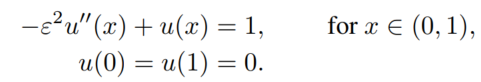
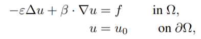
1D singular perturbation problem: singular perturbation problems are special cases where certain terms in the equations become disproportionately small or large, leading to different behaviors that are challenging to model. These problems often occur in many areas of science and engineering, such as fluid dynamics, electrical circuits, and control systems.

2D convection-dominated diffusion equation: this equation models physical phenomena where the convection effect (transport due to bulk motion) is much stronger than the diffusion effect (transport due to concentration gradients). These types of problems occur in various areas like meteorology (where wind disperses pollutants) and oceanography (where ocean currents transport heat).

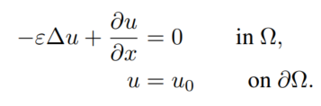
2D convection-dominated diffusion problem (featuring curved streamlines and an interior boundary layer): this is a more complex variant of the previous problem where the flow pattern is curved, and there is a significant boundary layer within the problem domain. These complications require a more sophisticated numerical approach and make the problem more representative of real-world challenges.

ε = 1e-4, Ω = (0, 1)², β = eˣ(sin(y), cos(y)).

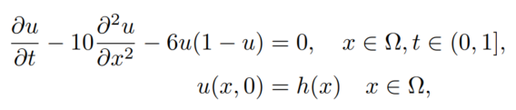
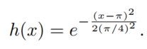
2D nonlinear reaction-diffusion equation (time-dependent): this equation models reactions combined with the diffusion of substances, but it’s also nonlinear and changes over time. These types of problems are common in fields like biology and chemistry, where substances interact and spread in a medium, and the reaction rates can change over time.

Ω = (0, 2π), periodic boundary conditions.

The benchmark studies yielded that:

the proposed algorithm showed substantial accuracy improvements across all test cases compared with naive PINNs;
the proposed algorithm showed robustness, with little sensitivity to the hyperparameter choices.

2.5 Strengths and Weaknesses

👍Strengths

Significantly improved accuracy compared to a single PINN.
Robust against the choice of network structure and arrangement.
Fewer efforts are required for fine-tuning hyperparameters.
Flexible and can be easily integrated with other PINNs techniques.

👎Weaknesses

Not suitable for solving conservation laws with derivative blow-ups (e.g., inviscid Burgers’ equation, Sod shock tube problem, etc.), which is due to the lack of sensitivity of these equations’ solutions to PDE loss.
Limitations in terms of scalability, as it may require more computational resources and time to train multiple neural networks in sequence.

2.6 Alternatives

Since this is the first paper that introduces the boosting algorithm to the PINN domain, there is currently no similar work as the current paper.

Nevertheless, in terms of enhancing the PINN’s capability of modeling challenging physical processes, the paper specifically mentioned the work of Krishnapriyan et al. There, the strategy is to divide the time domain into sub-intervals, and PINNs are built progressively to model each of the sub-intervals (similar to the idea covered in the previous blog).

The current paper compared Krishnapriyan’s approach with the newly proposed one in the last benchmark case study (section 2.4 above). The results showed that the proposed boosting approach is able to achieve 4 times lower error.

3 Potential Future Improvements

Further improvements of the proposed strategy include investigating the optimal sequential combination of the neural networks, mixing and matching with other types of neural network architectures in the gradient boosting training iterations, as well as integrating other best practices of PINN training (e.g., residual points generation) into the gradient boosting training framework.

4 Takeaways

In this blog, we looked at a new PINN training paradigm via boosting-based ensemble learning. This topic is highly relevant as it enhances PINNs’ capability to tackle challenging problems like multi-scale and singular perturbation problems.

As usual, here are the takeaways from the design pattern proposed in this paper:

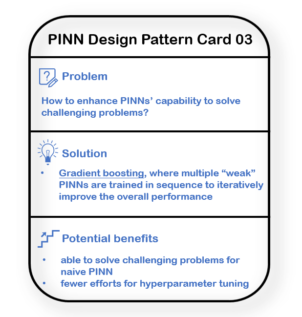
[Problem]: How to enhance PINNs’ capability to solve challenging problems?
[Solution]: Gradient boosting, where multiple “weak” PINNs are trained in sequence to iteratively improve the overall performance.
[Potential benefits]: 1. Able to solve challenging problems for naive PINN. 2. Fewer efforts for hyperparameter tuning

Here is another PINN design card:

PINN design pattern proposed in the paper. (Image by this blog author)

I hope you found this blog useful😃If you want to learn more about PINN design patterns, feel free to check out other posts in this series:

Looking forward to sharing more insights with you in the upcoming blogs!

Reference

[1] Fang et al., Ensemble learning for physics informed neural networks: a Gradient Boosting approach, arXiv, 2023.

[2] Krishnapriyan et al., Characterizing possible failure modes in physics-informed neural networks, arXiv, 2021.