Understanding the Mel Spectrogram

If you are anything like me, trying to understanding the mel spectrogram has not been an easy task. You read an article only to be lead to another… and another… and another… on and on it goes. I hope this short post will clarify some of the confusion and explain the mel spectrogram from the ground up.

Signals

A signal is a variation in a certain quantity over time. For audio, the quantity that varies is air pressure. How do we capture this information digitally? We can take samples of the air pressure over time. The rate at which we sample the data can vary, but is most commonly 44.1kHz, or 44,100 samples per second. What we have captured is a waveform for the signal, and this can be interpreted, modified, and analyzed with computer software.

import librosa
import librosa.display
import matplotlib.pyplot as plt

y, sr = librosa.load('./example_data/blues.00000.wav')

plt.plot(y);
plt.title('Signal');
plt.xlabel('Time (samples)');
plt.ylabel('Amplitude');

This is great! We have a digital representation of an audio signal that we can work with. Welcome to the field of signal processing! You may be wondering though, how do we extract useful information from this? It looks like a jumbled mess. This is where our friend Fourier comes in.

The Fourier Transform

An audio signal is comprised of several single-frequency sound waves. When taking samples of the signal over time, we only capture the resulting amplitudes. The Fourier transform is a mathematical formula that allows us to decompose a signal into it’s individual frequencies and the frequency’s amplitude. In other words, it converts the signal from the time domain into the frequency domain. The result is called a spectrum.

This is possible because every signal can be decomposed into a set of sine and cosine waves that add up to the original signal. This is a remarkable theorem known as Fourier’s theorem. Click here if you want a good intuition for why this theorems is true. There is also a phenomenal video by 3Blue1Brown on the Fourier Transform if you would like to learn more here.

The fast Fourier transform (FFT) is an algorithm that can efficiently compute the Fourier transform. It is widely used in signal processing. I will use this algorithm on a windowed segment of our example audio.

import numpy as np

n_fft = 2048
ft = np.abs(librosa.stft(y[:n_fft], hop_length = n_fft+1))

plt.plot(ft);
plt.title('Spectrum');
plt.xlabel('Frequency Bin');
plt.ylabel('Amplitude');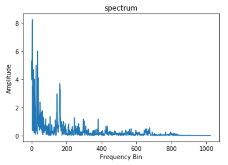

The Spectrogram

The fast Fourier transform is a powerful tool that allows us to analyze the frequency content of a signal, but what if our signal’s frequency content varies over time? Such is the case with most audio signals such as music and speech. These signals are known as non periodic signals. We need a way to represent the spectrum of these signals as they vary over time. You may be thinking, “hey, can’t we compute several spectrums by performing FFT on several windowed segments of the signal?” Yes! This is exactly what is done, and it is called the short-time Fourier transform. The FFT is computed on overlapping windowed segments of the signal, and we get what is called the spectrogram. Wow! That’s a lot to take in. There’s a lot going on here. A good visual is in order.

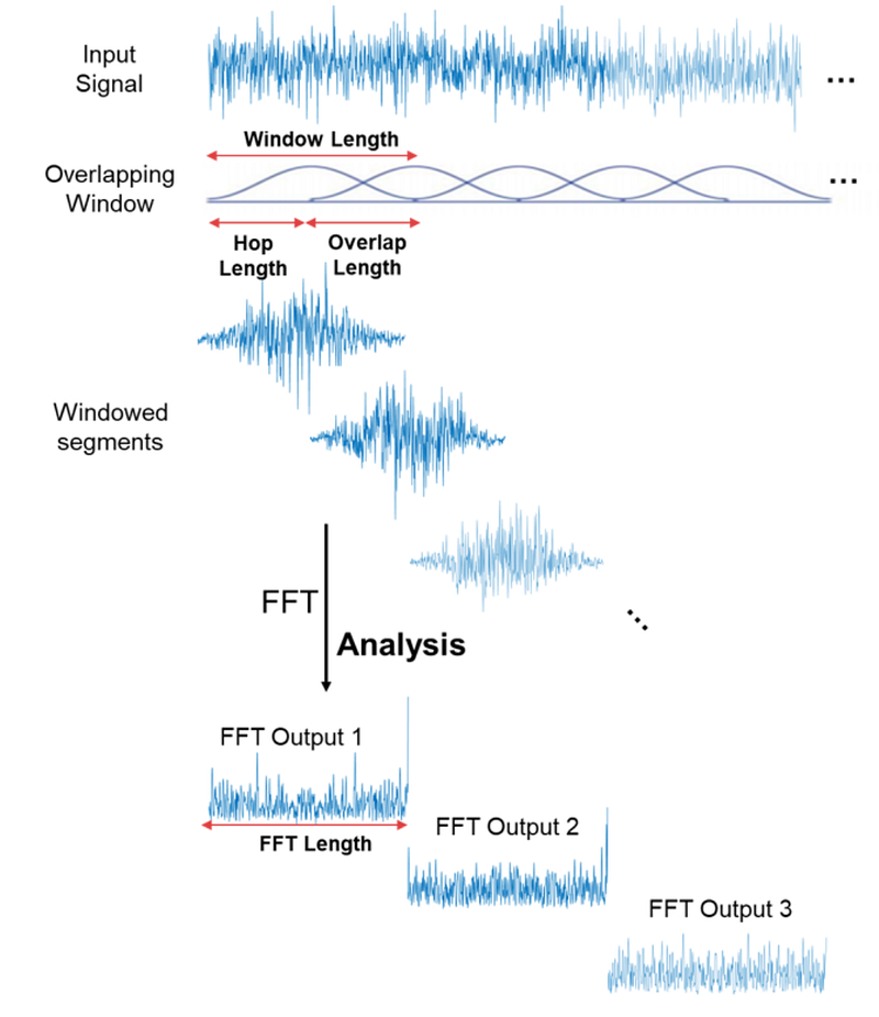
You can think of a spectrogram as a bunch of FFTs stacked on top of each other. It is a way to visually represent a signal’s loudness, or amplitude, as it varies over time at different frequencies. There are some additional details going on behind the scenes when computing the spectrogram. The y-axis is converted to a log scale, and the color dimension is converted to decibels (you can think of this as the log scale of the amplitude). This is because humans can only perceive a very small and concentrated range of frequencies and amplitudes.

spec = np.abs(librosa.stft(y, hop_length=512))
spec = librosa.amplitude_to_db(spec, ref=np.max)

librosa.display.specshow(spec, sr=sr, x_axis='time', y_axis='log');
plt.colorbar(format='%+2.0f dB');
plt.title('Spectrogram');

Voila! With only a couple lines of code, we have created a spectrogram. Ok. We are almost there! We have a solid grasp on the “spectrogram” part, but what about “Mel.” Who is he?

The Mel Scale

Studies have shown that humans do not perceive frequencies on a linear scale. We are better at detecting differences in lower frequencies than higher frequencies. For example, we can easily tell the difference between 500 and 1000 Hz, but we will hardly be able to tell a difference between 10,000 and 10,500 Hz, even though the distance between the two pairs are the same.

In 1937, Stevens, Volkmann, and Newmann proposed a unit of pitch such that equal distances in pitch sounded equally distant to the listener. This is called the mel scale. We perform a mathematical operation on frequencies to convert them to the mel scale.

The Mel Spectrogram

A mel spectrogram is a spectrogram where the frequencies are converted to the mel scale. I know, right? Who would’ve thought? What’s amazing is that after going through all those mental gymnastics to try to understand the mel spectrogram, it can be implemented in only a couple lines of code.

mel_spect = librosa.feature.melspectrogram(y=y, sr=sr, n_fft=2048, hop_length=1024)
mel_spect = librosa.power_to_db(spect, ref=np.max)

librosa.display.specshow(mel_spect, y_axis='mel', fmax=8000, x_axis='time');
plt.title('Mel Spectrogram');
plt.colorbar(format='%+2.0f dB');

In Summary

That was a lot of information to take in, especially if you are new to signal processing like myself. However, if you continue to review the concepts laid out in this post (and spend enough time staring at the corner of a wall thinking about them), it’ll begin to make sense! Let’s briefly review what we have done.

1. We took samples of air pressure over time to digitally represent an audio signal
2. We mapped the audio signal from the time domain to the frequency domain using the fast Fourier transform, and we performed this on overlapping windowed segments of the audio signal.
3. We converted the y-axis (frequency) to a log scale and the color dimension (amplitude) to decibels to form the spectrogram.
4. We mapped the y-axis (frequency) onto the mel scale to form the mel spectrogram.

That’s it! Sounds easy, right? Well, not quite, but I hope this post made the mel spectrogram a little less intimidating. It took me quite a while to understand it. At the end of the day though, I found out that Mel wasn’t so standoffish.

If you would like to see a cool application of this topic, check out my post on musical genre classification where I use mel spectrograms to train a convolutional neural network to predict the genre of a song. How does it do? Find out here!