Musical Genre Classification with Convolutional Neural Networks

As a lover of both music and data, the idea of combining the two sounded enticing. Innovative companies such as Spotify and Shazam have been able to leverage music data in a clever way to provide amazing services to users! I wanted to try my hand at working with audio data and try to build a model that could automatically classify a song by its genre. The code for my project can be found here.

An automatic genre classification algorithm could greatly increase efficiency for music databases such as AllMusic. It could also help music recommender systems and playlist generators that companies like Spotify and Pandora use. It’s also a really fun problem to play around with if you love music and data!

There are two major challenges with this problem:

1. Musical genres are loosely defined. So much so that people often argue over the genre of a song.
2. It is a nontrivial task to extract differentiating features from audio data that could be fed into a model.

The first problem we have no control over. This is the nature of musical genres, and something that will be a limitation. The second problem has been heavily researched in the field of Music Information Retrieval (MIR), which is dedicated to the task of extracting useful information from audio signals.

If you take the time to really think about it, this is a hard problem! How do we turn vibrations in air pressure into information we can gain insights from?

I spent a lot of time researching this question. In order to build a model that could classify a song by its genre, I needed to find good features. An interesting feature that kept coming up was the mel spectrogram.

The Mel Spectrogram

The mel spectrogram can be thought of as a visual representation of an audio signal. Specifically, it represents how the spectrum of frequencies vary over time. I wrote an article (here) that goes into depth on this topic if you would like to learn more. For the tl;dr folks out there, here is a brief summary:

The Fourier transform is a mathematical formula that allows us to convert an audio signal into the frequency domain. It gives the amplitude at each frequency, and we call this the spectrum. Since frequency content typically varies over time, we perform the Fourier transform on overlapping windowed segments of the signal to get a visual of the spectrum of frequencies over time. This is called the spectrogram. Finally, since humans do not perceive frequency on a linear scale, we map the frequencies to the mel scale (a measure of pitch), which makes it so that equal distances in pitch sound equally distant to the human ear. What we get is the mel spectrogram.

The best part? It can be generated with only a few lines of code in Python.

import librosa

y, sr = librosa.load('./example_data/blues.00000.wav')

mel_spect = librosa.feature.melspectrogram(y=y, sr=sr, n_fft=2048, hop_length=1024)
mel_spect = librosa.power_to_db(spect, ref=np.max)

librosa.display.specshow(mel_spect, y_axis='mel', fmax=8000, x_axis='time');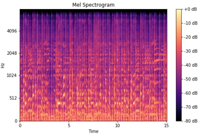

Pretty amazing, huh? We now have a way to visually represent a song. Let’s take a look at some mel spectrograms from songs of different genres.

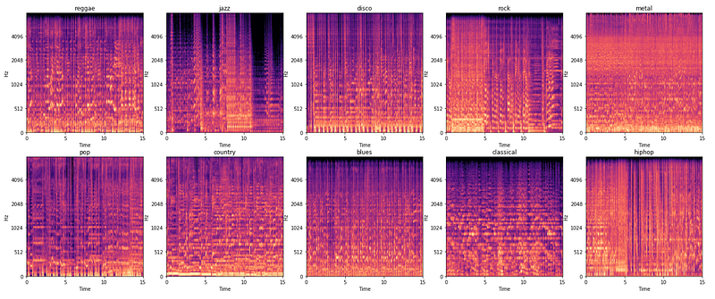
This is awesome! Some of the idiosyncratic differences in genres are captured in the mel spectrogram, which means they could make great features.

What we have essentially done is turned the problem into an image classification task. This is great because there’s a model that was made specifically for this task: the convolutional neural network (CNN). This leads me to the main question of my project: how accurate can a convolutional neural network identify musical genres using mel spectrograms?

Let’s get into it!

Gathering and Preprocessing the Data

The dataset I used was the GTZAN Genre Collection (found here). This dataset was used in a well known paper on genre classification in 2002. The dataset includes 10 different genres (blues, classical, country, disco, hip hop, jazz, metal, pop, reggae, and rock) with 100 songs per genre (each 30 second samples). Since they were all .wav files, I was able to use the librosa library to load them into a Jupyter Notebook.

As seen above, computing the mel spectrogram using librosa is fairly straightforward. I was able to write a function that computes the mel spectrogram for each audio file and stores them in a numpy array. It returns that array as well as an array with the corresponding genre labels.

Now that we have our features and targets, we can create a holdout, or validation, set. I chose to hold out 20% for testing.

Before constructing the model, a few steps have to be taken:

1. Values of the mel spectrograms should be scaled so that they are between 0 and 1 for computational efficiency.
2. The data is currently 1000 rows of mel spectrograms that are 128 x 660. We need to reshape this to be 1000 rows of 128 x 660 x 1 to represent that there is a single color channel. If our image had three color channels, RGB, we would need this additional dimension to be 3.
3. Target values have to be one-hot-encoded in order to be fed into a neural network.

It is important that we complete these steps after creating our holdout set to prevent data leakage. Now we are ready to do some modeling!

How Did the CNN do?

Before running a CNN, I wanted to train a feed forward neural network (FFNN) for comparison. CNNs have additional layers for edge detection that make them well suited for image classification problems, but they tend to be more computationally expensive than FFNNs. If a FFNN could perform just as well, there would be no need to use a CNN. Since the main focus of this post is the CNN, I won’t go into the details of the model here, but the best FFNN model achieved a test score of 45%.

As suspected, the CNN model did much better! The best CNN model (based on test score accuracy) achieved a score of 68%. That’s not too shabby, especially considering the difficulty of the problem, but it still isn’t great. The training score was 84%, so the model was overfit. This means that it was tuning really well to the training data and not generalizing as well to new data. Even so, it’s certainly learning.

I tried several different architectures to try to improve the model, and most of them achieved accuracies between 55 and 65 percent, but I couldn’t get it much above that. Most of the models became increasingly overfit after about 15 epochs, so increasing the number of epochs did not seem like a good option.

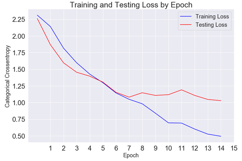
Here is a summary of the final architecture:

1. Input layer: 128 x 660 neurons (128 mel scales and 660 time windows)
2. Convolutional layer: 16 different 3 x 3 filters
3. Max pooling layer: 2 x 4
4. Convolutional layer: 32 different 3 x 3 filters
5. Max pooling layer: 2 x 4
6. Dense layer: 64 neurons
7. Output layer: 10 neurons for the 10 different genres

All of the hidden layers used the RELU activation function and the output layer used the softmax function. The loss was calculated using the categorical crossentropy function. Dropout was also used to prevent overfitting.

A Deeper Look

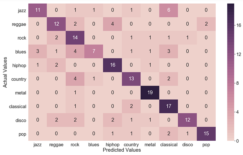
To look deeper into what was happening with the model, I computed a confusion matrix to visualize the model’s predictions against the actual values. What I found was really interesting!

Blues or Jazz?

The model hardly ever predicted blues, and only correctly classified 35% of blues songs, but a majority of the misclassifications were jazz and rock. This makes a lot of sense! Jazz and blues are very similar styles of music, and rock music was heavily influenced by, and really came out of, blues music.

Reggae or Hiphop?

The model also had a tough time distinguishing between reggae and hiphop. Half of the misclassifications for reggae were hiphop and vise versa. Again, this makes sense since reggae music heavily influenced hiphop music and share similar characteristics.

Is This Rock?

The model misclassified several genres as rock, particularly blues and country. It’s no wonder though because there are so many sub-genres of rock music that branch into other genres. Blues rock is very popular as well as southern rock which has country influences.

What Does This Tell Us?

This is actually really good news! Our model is running into the same difficulties that a human would. It’s clearly learning some of the distinguishing factors of the musical genres, but it is having trouble with genres that share characteristics with other genres. Again, this goes back to the first problem, and that is the nature of musical genres. They are difficult to distinguish!

Even so, I’d say that for a computer, 68% accuracy isn’t all that bad, but I do believe there’s room for improvement. I can confidently say that the CNN did better than the FFNN, and that it was able to learn and predict with decent accuracy the genre of a song.

A Natural Question

What happens if we remove some of the genres that share characteristics with other genres? Will the model perform better? How does it do with a binary classification? These were some of the questions still burning in my mind. If you’d like to dive deeper into these questions, stay tuned for my next post.

To be continued…