Tutorial on DFT Studies of 1D Nanomaterials Using Quantum Espresso

This tutorial is for beginners who are interested in learning how to set up and run a first-principle calculation based on density functional theory (DFT). DFT is the most widely used method by quantum chemists, condensed matter physicists, and material scientists for calculating important materials properties such as equilibrium geometry, quantum energy levels, optoelectronic properties, vibrational properties, IR spectrum, etc.

DFT can be used for both molecular systems (finite size) or extended periodic systems like solids. Here we focus on DFT calculations for 1D periodic systems. As an example, we consider an armchair graphene nanoribbon (AGNR) with N = 7 dimer lines. To find out about setting up and running a DFT calculation for a molecule or polymer, see the following: Tutorial on Density Functional Theory using GAMESS. For DFT studies for 2D layered materials, see the following: Tutorial on Density Functional Theory using quantum espresso.

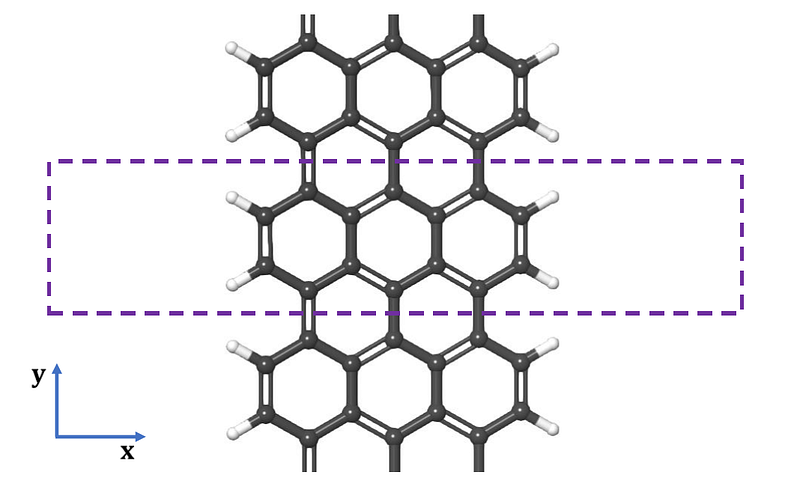
For practical purposes, we consider only a self-consistent field calculation at fixed equilibrium geometry. A geometry optimization calculation can be performed by selecting ‘relax’ under the calculation key, or ‘vc-relax’ if the unit cell has to be optimized as well. For 1D systems, vacuum regions must be added to the other two dimensions to avoid interaction between edges and planes, as shown in the figure above.

A self-consistent calculation is first performed using atomic pseudopotentials to obtain the converged electron density, which is then used to calculate the quantum energy levels of the system. A band structure calculation is performed at the end of the self-consistent field calculation in order to predict important optoelectronic parameters such as energy band gap and electron/hole effective masses. All calculations are performed using the Quantum Espresso DFT Solver. For more information, see the following link: https://www.quantum-espresso.org/.

You can download off-the-shelf input files for performing DFT calculations for 1D systems such as a graphene nanoribbon (GNR) from this repository: https://github.com/bot13956/Tutorial_DFT_1D_Nanomaterials_QuantumEspresso.

Necessary Components of the Calculation

1. Atomic Pseudopotential files:

H.pz-rrkjus_psl.1.0.0.UPF: atomic pseudopotential file for Hydrogen.

C.pz-n-rrkjus_psl.0.1.UPF: atomic pseudopotential file for Carbon.

There are several websites where you can find pseudopotential files, for e.g. http://www.quantum-espresso.org/pseudopotentials.

When downloading a pseudopotential file, remember that the naming convention for each file reveals the type of exchange-correlation potential (LDA = Local Density Approximation, GGA = Generalized Gradient Approximation, hybrid, etc) that was used in generating the file, as well as the pseudopotential type (NC = Norm-Conserving, PAW = Projector-Augmented Wave, and US = Ultrasoft). If your calculation is going to take relativistic effects (important for systems containing high-Z atoms) into consideration, make sure you understand the difference between scalar relativistic and full relativistic pseudopotentials. For example, the pseudopotential files listed above for the elements H, and C are scalar-relativistic ultrasoft LDA pseudopotentials. In general and depending on the system, hybrid pseudopotentials perform better than GGA pseudopotentials, and GGA pseudopotentials perform better than LDA pseudopotentials.

2. Input file for performing self-consistent field calculations

scf.in: performs self-consistent field calculations using density functional theory.

3. Input file for performing non-self-consistent field calculations

nscf.in: performs band structure calculation after self-consistent field calculation is completed to determine quantized energy levels and Fermi energy.

4. Input file for calculating the energy eigenvalues and eigenfunctions

bands.in: performs band structure calculation after self-consistent field calculation is completed. Band structure is computed along a given path joining high symmetry points in first Brillouin Zone.

5. Input file for generating band structure as a one-dimensional plot

bands_plot.in: re-order and re-arrange band structure data into a format suitable for plotting.

6. Batch script file for scheduling (if running calculations on a cluster)

batch_script.sl: batch script for batch scheduling and allocating of computer resources.

Analysing Results from a Band Structure Calculation

A band structure calculation provides useful information such as:

1. Band structure plot (direct or indirect semiconductor).
2. Density of states (from which we can infer if a material is an insulator, semiconductor, or metal).
3. Energy band gap (for optoelectronic applications).
4. Carrier effective mass (for applications in charge transport and thermoelectricity).

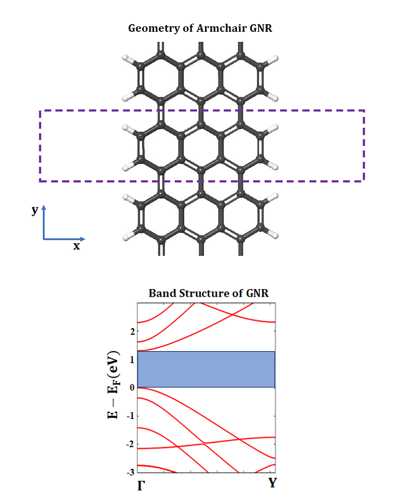
The figure below shows is the band structure of an AGNR with N = 7 dimer lines. It shows a direct band gap with value of 1.305 eV. If the ions and unit cell are relaxed using a ‘vc-relax’ calculation before performing a band structure calculation, an improved band gap of 1.603 eV is obtained.

In summary, we have provided a tutorial that can help beginners to set up and run a DFT calculation for periodic systems. For more information on how to create various input files as well as tuning different hyperparameters such as convergence criteria, see the quantum espresso input file description documentation: https://www.quantum-espresso.org/Doc/INPUT_PW.html.

References

1. P. Giannozzi et al., J. Phys.:Condens. Matter 21 395502 (2009).
2. P. Giannozzi et al., J. Phys.:Condens. Matter 29 465901 (2017).
3. Quantum Espresso URL: http://www.quantum-espresso.org.
4. NERSC for supercomputing resources: https://www.nersc.gov/.