Machine Learning

Training a Machine Learning Model on a Dataset with Highly-Correlated Features

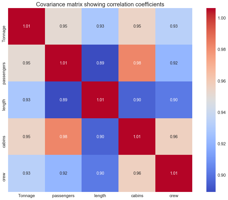
In the previous article (Feature Selection and Dimensionality Reduction Using Covariance Matrix Plot), we’ve shown that a covariance matrix plot can be used for feature selection and dimensionality reduction.

Using the cruise ship dataset cruise_ship_info.csv, we found that out of the 6 predictor features [‘age’, ‘tonnage’, ‘passengers’, ‘length’, ‘cabins’, ‘passenger_density’], if we assume important features have a correlation coefficient of 0.6 or greater with the target variable, then the target variable “crew” correlates strongly with 4 predictor variables: “tonnage”, “passengers”, “length, and “cabins”.

We, therefore, were able to reduce the dimension of our feature space from 6 to 4.

Now, suppose we want to build a model on the new feature space for predicting the crew variable. Our model can be expressed in the form:

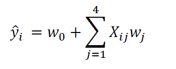
where X is the feature matrix, and w the weights to be learned during training.

Looking at the covariance matrix plot between features, we see that there is a strong correlation between the features (predictor variables), see the image above.

How do we deal with the problem of correlations between features?

In this article, we shall use a technique called Principal Component Analysis (PCA) to transform our features into space where the features are independent or uncorrelated. We shall then train our model on the PCA space. You may find out more about PCA from this article: Machine Learning: Dimensionality Reduction via Principal Component Analysis.

Training the Model on the PCA Space

1. Import necessary libraries

import numpy as np
import pandas as pd
import matplotlib.pyplot as plt
import seaborn as sns

2. Read dataset and display columns

df=pd.read_csv("cruise_ship_info.csv")
df.head()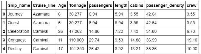

3. Selecting important variables (columns)

cols_selected = ['Tonnage', 'passengers', 'length', 'cabins','crew']
  
df[cols_selected].head()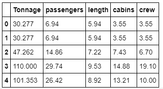

4. Data partitioning into training and testing sets

from sklearn.model_selection import train_test_split
X = df[cols_selected].iloc[:,0:4].values     
y = df[cols_selected]['crew']

X_train, X_test, y_train, y_test = train_test_split( X, y, test_size=0.4, random_state=0)

5. Build multiple linear regression model on PCA space

from sklearn.preprocessing import StandardScaler
from sklearn.decomposition import PCA
from sklearn.linear_model import LinearRegression
from sklearn.pipeline import Pipeline
from sklearn.metrics import r2_score

train_score = []
test_score = []
cum_variance = []

for i in range(1,5):
    X_train, X_test, y_train, y_test = train_test_split( X, y, test_size=0.4, random_state=0)
    y_train_std = sc_y.fit_transform(y_train[:, np.newaxis]).flatten()
    
    pipe_lr = Pipeline([('scl', StandardScaler()),
                        ('pca', PCA(n_components=i)),
                        ('slr',   LinearRegression())]) 

    pipe_lr.fit(X_train, y_train_std)

    y_train_pred_std = pipe_lr.predict(X_train)
    y_test_pred_std = pipe_lr.predict(X_test)
    y_train_pred=sc_y.inverse_transform(y_train_pred_std)
    y_test_pred=sc_y.inverse_transform(y_test_pred_std)

    train_score = np.append(train_score, 
                            r2_score(y_train, y_train_pred))

    test_score = np.append(test_score, 
                           r2_score(y_test, y_test_pred))

    cum_variance = np.append(cum_variance, np.sum(pipe_lr.fit(X_train, y_train).named_steps['pca'].explained_variance_ratio_))

Here is the output from the Regression Model on PCA Space:

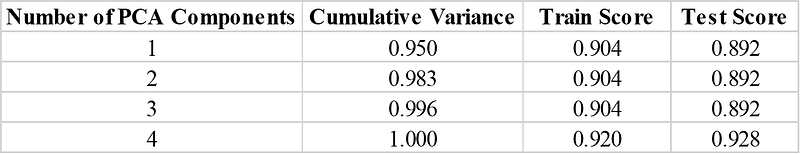
Based on this summary, we see that 95 percent of the variance is contributed by the first principal component alone. This means that in the final model, only the first principal component PC1 could be used since the other 3 components PC2, PC3, and PC4 contribute only about 5% of the total variance.

PCA for dimensionality reduction doesn’t seem like a big deal for a dataset with 4 features, but for a complex dataset having hundreds or even thousands of features, PCA can be a powerful tool that can be used for removing correlation between features and helps to decrease the computational time for model training, testing, and evaluation.

In summary, we have shown how the PCA algorithm can be implemented using python’s sklearn package with the cruise ship dataset. PCA is such a powerful tool for model building, especially when dealing with a complex dataset with highly-correlated features. You can download the entire dataset and code for this article on Github.

References

1. Raschka, Sebastian, and Vahid Mirjalili. Python Machine Learning, 2nd Ed. Packt Publishing, 2017.
2. Benjamin O. Tayo, Machine Learning Model for Predicting a Ships Crew Size, https://github.com/bot13956/ML_Model_for_Predicting_Ships_Crew_Size.