Summary

The web content provides a tutorial on basic time series analysis using Python and pandas, focusing on data cleaning, date-time manipulation, and visualization with real-world financial data from Reliance Global Group Inc.

Abstract

The article "Time Series Analysis with Python" introduces readers to fundamental techniques for analyzing temporal data within a pandas DataFrame. It guides the audience through downloading historical stock data of Reliance Global Group Inc, cleaning the data by removing dollar signs and converting string values to floats, and setting the date as an index for time series analysis. The tutorial emphasizes the importance of foundational skills in time series analysis, particularly for those in the finance sector who are increasingly expected to complement their financial expertise with programming skills. The article also demonstrates how to resample data to visualize trends on a monthly and weekly basis using matplotlib for plotting. The author concludes by acknowledging that the article covers only the basics and encourages readers to reach out via LinkedIn or Twitter for further engagement.

Opinions

The author believes that a strong foundation in basic time series analysis is crucial for more advanced financial data analysis.
There is an emphasis on the growing expectation for financial analysts to be proficient in programming, particularly Python, to leverage advanced technologies in finance.
The article suggests that statistics and machine learning are key drivers in the growth and advancement of the finance sector.
The author expresses that the process of data cleaning and preprocessing constitutes a significant portion (60-70%) of the ETL (Extract, Transform, Load) process in time series analysis.
By providing a link to the author's LinkedIn and Twitter profiles, the author encourages reader interaction and further discussion on the topic.

Data Visualization

Time Series Analysis with Python

Date and Time analysis on a data frame with pandas

Time series analysis is dealing with date and time index points in the data frame. The most frequent use of time series in the finance field. This article will help people who always analyze data with respect to date and time. Well for time series analysis, we need a skilled analyst who knows the forecasting evaluation. Financial analysts are now very skilled with programming also rather analyze in a classical way. How statistics and machine learning helps the finance sector to grow with advanced technologies around us.

This article deals with only basic analysis w.r.t date and time. Big analysis needs foundation skills first. Hope you will feel interested in this article.

Download the Reliance Global Group Inc ( RELI ) historical data from here. From this link, you can download all other historical data and it is available. I Downloaded the RELI CSV datasheet for six months for educational analysis purposes. In this article, we will learn some basic concepts of time series with python.

For analysis, we will use a jupyter notebook of anaconda distribution. We change the name of the sheet to reli_data.

Z- Statistics, T-Statistics, P-Statistics are Still Confusing you?

Definitions and concepts in Statistics for machine learning

medium.com

The Data look like this

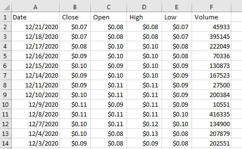
The columns names are Date, Close, Open, High, Low and Volume.

Open the jupyter notebook and need to import the library to read the CSV file. When reading the CSV file, sometimes there are spaces after delimiter, to remove them we use ‘skipinitialspace=True’ while reading the CSV file.

#importing the library
import pandas as pd
#reading the csv file and save it to data variable
data = pd.read_csv('reli_data.csv', skipinitialspace=True)
#view the data up to 5 rows
data.head()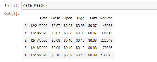

If we noticed in the data we have a dollar sign and we have to remove it for analysis on integer only. We have four columns with dollar signs.

#removing dollar sign 
data['Close'] = data['Close'].str.replace('$', '')
data['Open'] = data['Open'].str.replace('$', '')
data['High'] = data['High'].str.replace('$', '')
data['Low'] = data['Low'].str.replace('$', '')

#view updated dataframe
data.head()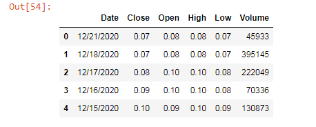

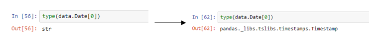
Dollar sign are removed in the column’s value. A photo by Author

Now check the type of the Date column and it comes to be a string and new want it to be a date column so for this, we need to parse the date column as a ‘date’ while reading with CSV file.

Type of date column changed. A photo by Author

Sometimes when we work on time series we need date as an index. To change the default index to Date as an index we use set_index function.

data.set_index("Date", inplace = True)
data.head()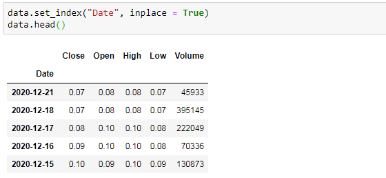

Another thing came across while accessing the columns which had dollar signs. There were still str values after removing the dollar sign. So, we also need to change these columns to float values as they have decimal points in them.

#value before converting
type(data.Low[0])
#output: str

#converting str values of column to float values
data["Close"] = pd.to_numeric(data["Close"], downcast="float")
data["Open"] = pd.to_numeric(data["Open"], downcast="float")
data["High"] = pd.to_numeric(data["High"], downcast="float")
data["Low"] = pd.to_numeric(data["Low"], downcast="float")

#to check after converting
type(data.Low[0])

#output: numpy.float32

Sometimes we see graph changes with the date as day, week, month or even year wise. To have a such chart we are taking the mean of the column as month-wise and let’s see. We use matlotlip for visualization.

#Month wise
%matplotlib inline
data.Open.resample('M').mean().plot()
#Week wise - just to change it to W(Week)
data.Open.resample('W').mean().plot()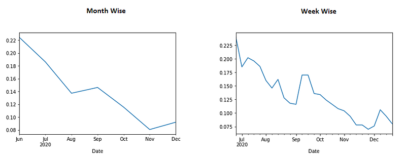

Open Value graph of RELI data records monthly and weekly wise. A photo by Author

Conclusion:

This article is only a basic understanding of time series analysis. The good point in this article is we downloaded the raw data and the did data cleaning part that we are facing a 60–70% ETL process.