
Statistics
Z- Statistics, T-Statistics, P-Statistics are Still Confusing you?
Definitions and concepts in Statistics for machine learning

Understanding statistics look like a side parallel road for data science and machine learning people. But learning statistics is worth making the inferences and solutions from the data. The road not to be taken by many people should have to accept the statistics with their daily dose. Well, in this article we will discuss the Z, T and P statistics distribution and will try to learn why we use them in data science. Before diving into this concept we will discuss some basic definition and terms as shown below:
Topics to be covered:
Section 1: Types of Data, Histogram and Scatter plot
Section 2: Central Measures values and Measures of Spread
Section 3: Covariance and Correlation
Section 4: Z, T — Distributions and confidence intervals
Section 5: Hypothesis and P — Distribution
Section 1:
Types of Data
Acquiring knowledge about statistics is a need in a data science career. Before jumping we should know with whom we are dealing with oh! that is obvious “DATA”. It is not like that data will come to you and tell all the inferences, we need to find a way to deal with different types of data.
Data is comprised of numbers and words that can be in the measurable or observational form. We cannot do the same operation with all different types of data, for this we need to identify and according to that, we need to test and visualize.
Numerical Data: This type of data deals with numbers which can be in a quantitative form either discrete or in continuous.
- Discrete data is like a whole number ( 2, 10, 20, 15, etc) which tells a direct specification of the quantity that we count easily.
- Continuous data is like a range means the value which falls in some particular measuring range ( Kg, Km, cm, etc ).
Categorical Data: This type deals with qualitative data that we can describe. It comes in a group of two or more types of a different description.
Example: Binary values ( 0 and 1 ),
Nominal Data: They are not in order but shows some groups or category like seasons, brand names, flower names, etc.
Ordinal Data: Well these types of data are those where we give them some rating or in some order.
Histogram and Scatter plot
If data is very big then we cannot sit all day and check every line of data records to take out some information. That’s where graphs and plots of data come into the picture.
Different types of plots are Bar, Line and Pie Charts, Histogram and Scatter plots, etc.
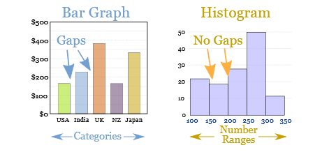
Histogram
Histograms although similar to bar charts but in the histogram, the bar falls in some range i.e. continuous type. The bar charts can have a gap between two bars but histogram doesn’t.
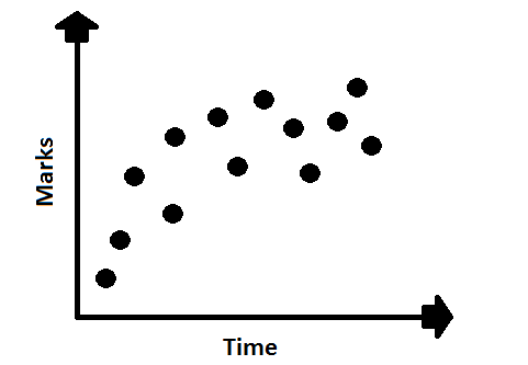
Scatter Plot
The scatter plot shows the relationship between two variable points in the record.
Section 2:
Central Measures value
When we want to know about something from a big record we choose one thing which is similar to all others. So, in numbers, we choose a common and around value through Mean, Median and Mode.
Measures of Spread
The Range
When we arrange the data in ascending order and make a difference from the big number to a small number is called range.
Mean Deviation
This spread tells us how far the values from the measured central value.
- First, take a mean of the values.
- Then make a difference from the mean value to all values.
- Then calculates the spread distance from the mean.
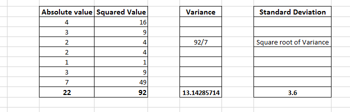
Example:
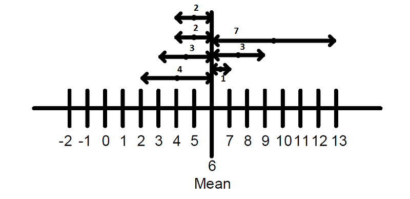
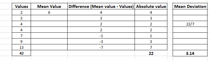
Mean Deviation = (4+3+2+2+1+3+7)/7 = 3.14
The mean deviation tells that on average the values are 3.14 far away from the middle.
Variance and Standard Deviation
Variance is the average of the sum of the squared of absolute values. It tells how the data is spread around the mean.
Standard deviation is how to spread if from the simple mean.
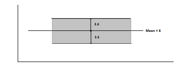
If we see in the photo the 6+3.6 is 9.6 and 6-3.6 is 2.4 so, we can say that numbers from 2.4 to 9.6 are in standard but if we see that the value 13 is outside the standard value range. From this, we can observe which numbers are very small or very big.
Section 3:
Covariance
Covariance is used to calculate the movement of the two variables. With the result, we can say that both variables are moving together, opposite or independent of each other. A positive value means moving together, negative values moving opposite and equal to zero means both are independent of each other.
Covariance > 0 → moving together
Covariance < 0 → moving opposite
Covariance = 0 → independent to each other
The formula to calculate covariance is
Covariance ( sample ) = Sum of (( x-x mean ) * ( y-y mean ))/n-1
The value can come in any scale from 0.000824 to 23,434,000 to interpret these types of values we do correlation coefficient.
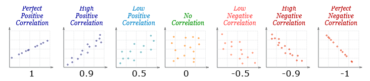
Correlation
Correlation is used to know the relationship between two variables.
The following types are the correlation shown in the photo below:
Section 4:
Distribution is the probability that we measure and see the probability distribution through graphs that’s how we see inferential statistics.
Normal Distribution
The normal distribution is sometimes called Gaussian Distribution in statistics terms. Many people also say this distribution is a bell curve because the mean, median and mode are equal and symmetrical with no skew.
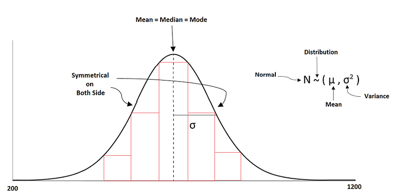
The spread of the curve is defined by the standard deviation. We can observe that more number of the observations or values are in the middle means around the mean. If we change the mean to a smaller and larger value then we see the distribution will shift towards right and left. If we change the standard deviation then the distribution becomes wider or narrower. The narrower means most of the observation around the center.
Z— Distributions
The changes we see in the distribution by changing mean and standard deviation are not stable. So, we need to standardize it so that we can calculate and make inferences. To make it standardize we have to make the mean to “0” and Standard deviation to “1” i.e ( 0, 1 ). To standardize we calculate the z score as shown below:
z = (value — mean)/standard deviation
When we calculate the mean and standard deviation of all z values it comes around 0 and 1 only obtaining a standard normal distribution.
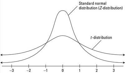
T — Distribution
It is generally called Student’s t distribution used to inference from the small sample with unknown variance. The difference between the normal distribution and t-distribution through the graph is t-distribution has a higher dispersion on the left and right sides of the distribution.
The formula for t-distribution is
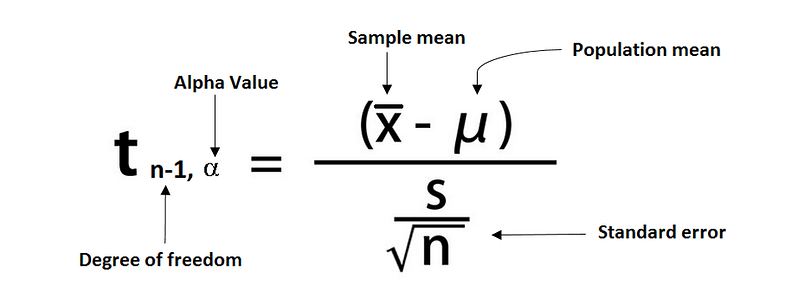
In a common thumb table, we use a t-distribution table up to 50 samples, if the sample size more than 50 then use a z-distribution table.
The degree of freedom is the one less of a total number of samples. Alpha is the percentage left after the confidence level percentage.
Confidence interval
When we do some estimation value for a population to be exact but with a practical approach, it comes wrong. So, we go for the confidence interval for a particular value to be in that range.
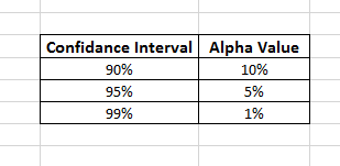
We see in the photo that we can choose a confidence interval with these common values and with respect to their alpha values.
Section 5:
Hypothesis
When we estimated the correct confidence interval, we try to find the value in that range, this need to make a decision. The hypothesis test to be done based on some points.
- Formulate a hypothesis
- Need the right test to be done
- Execute the test
- Make a decision
A hypothesis is just think or idea on which we do testing. There are two types of hypotheses.
- Null hypothesis
- Alternate hypothesis
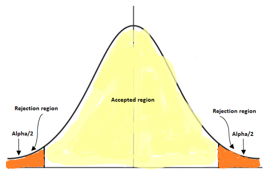
The null hypothesis is the one which we think about to be a parameter and the rest is an alternate hypothesis. When we calculate the Z value for the hypothesis then we also calculate the significance value also based on alpha. The confidence interval on the distribution and divide the alpha value for both left and right sides.
P — Distribution
P- value gives the smaller significance level on which we can reject the null hypothesis on sample data.
Conclusion:
A basic understanding of statistics can give valuable information in data science. Believe me statistics in not boring. when you try to learn with practical examples it will do magic for you. As statistics is a very vast subject so, I tried to give some basic ideas. Hope this article will give a little interesting for readers.
I hope you like the article. Reach me on my LinkedIn and twitter.


