The Technical Interview Guide to Backtracking

A JavaScript guide to backtracking for interview prep and daily coding

In a previous article, we discussed dynamic programming, which is a method to solve a larger problem by building up a solution solving smaller subproblems. It uses optimal substructure.

In this article, we are going to focus on another hot topic: backtracking.

Backtracking is a general algorithm for finding all or some solutions to a computational problem that incrementally builds candidates to the solutions while abandoning each partial candidate (backtracks). A partial candidate is abandoned either because it cannot possibly be completed to a valid solution or because the problem needs to find all valid solutions.

What are the differences between dynamic programming and backtracking?

Dynamic programming emphasizes on overlapping subproblems, while backtracking focus on all or some solutions.
Dynamic programming relies on the principle of optimality, while backtracking uses a brute force approach.
Dynamic programming is more like breadth-first search (BFS), building up one layer at a time, while backtracking is more like depth-first search (DFS), building up one solution first.
Dynamic programming usually takes more space than backtracking, by memoizing all the optimal sub-solutions for later use.
Backtracking usually takes more time to execute, by iterating all or some solutions.

Some problems can be optimized by dynamic programming, and some problems are easier for backtracking. It is applied to different situations case by case.

In this article, we are going to go over a few backtracking problems.

A Typical Backtracking Structure

We try to standardize the backtracking solution:

Name the backtrack function as backtrack.
Put backtrack inside the function to take the advantage of closure.
The following is the structure of a typical backtrack algorithm:

Permutations, Combinations, Subsets, and Variations

Permutations

A permutation of a set is an arrangement of its members into a sequence. The order of selection matters. To use [1, 2, 3] as an example, its permutations are [[1, 2, 3], [1, 3, 2], [2, 1, 3], [2, 3, 1], [3, 1, 2], [3, 2, 1]].

Here is the backtracking algorithm to print out permutations from number choices:

At line 28, we try the next candidate using the original start value, which will use every candidate. To prevent the same choice being used more than once, line 23 ensures that the number has not been used yet.

The algorithm’s time complexity is O(n⋅n!), because there are n! different permutations and each one has n numbers to be copied into the answer.

The algorithm’s space complexity is O(n), because the depth of the call stack is equal to the number length.

These are verifying tests:

Permutation Count

Obviously, we can use dynamic programming for the optimal solution if the problem only asks for the permutation count.

Here is the dynamic programming algorithm to print out permutation count from number choices:

The algorithm’s time complexity is O(n), and space complexity is O(n).

These are verifying tests:

Not surprisingly, the permutation count is the factorial number.

Combinations

A combination is a selection of items from a collection. The order of selection does not matter. We can use a similar program to calculate the combinations. [1, 2, 3]’s combinations with length 2 are [[1, 2], [1, 3], [2, 3]].

Here is the backtracking algorithm to compute combinations from number choices with specific length:

At line 27, we try the next candidate using i + 1, which will start with an unused candidate.

The algorithm’s time complexity is

The algorithm’s space complexity is O(m).

These are verifying tests:

Subsets

Set A is a subset of set B if all elements of A are also elements of B. It is possible for A and B to be equal. For example, [1, 2, 3] has subsets [[],[1], [1, 2], [1, 2, 3], [1, 3], [2], [2, 3], [3]]. One of the subsets, [1, 2, 3], is itself.

Here is the backtracking algorithm to print out subsets from number choices:

The algorithm’s time complexity is

The algorithm’s space complexity is O(n).

These are verifying tests:

Permutation Subsets

The subsets are combinations. How about treat a subset’s permutations differently? Use [1, 2] as an example:

Its subsets are [[], [1], [1, 2], [2]].
Its permutation subsets are [[], [1], [1, 2], [2], [2, 1]].

To generate permutation subsets, each backtracking call needs to start from the first choice. Also, the used choice can not be reused.

Here is the algorithm for permutation subsets:

Lines 24 - 26 backtrack from unused choices.

The algorithm’s time complexity is

The algorithm’s space complexity is O(n).

These are verifying tests:

Permutation Subsets Not Unique

We have assumed that each number choice is a unique natural number. What if the number choices are not unique?

For example, [1,2,1]’s permutation subsets are [[],[1],[1,1],[1,1,2],[1,2],[1,2,1],[2],[2,1],[2,1,1]].

In this case, we need to sort the choices to make sure the same numbers are next to each other. Therefore, we can avoid putting the same number at the same position multiple times.

Here is the algorithm for permutation subsets with numbers that are not unique:

Line 46 sorts the choices.

Lines 32 - 37 skip the choices that are the same as the previous ones.

The algorithm’s time complexity is

The algorithm’s space complexity is O(n).

These are verifying tests:

Combinational sum with no duplicates

Provided with an array of distinct natural number choices and a target value, we can use a combination algorithm to find unique combinations that sum up to the target value. Each number choice can be used at most once. For example, the choices are [1, 2, 3, 4] and the target is 5. The unique combinations are [[1, 4], [2, 3]].

The backtracking algorithm for no-duplicate combinations is written as follows:

The algorithm’s time complexity is

The algorithm’s space complexity is O(n).

These are verifying tests:

Combinational sum with duplicates

We change the condition to allow each number choice to be used as many times as possible. For the same example of choices [1, 2, 3, 4] and the target of 5. The allow-duplicate combinations are [[1, 1, 1, 1, 1], [1, 1, 1, 2], [1, 1, 3], [1, 2, 2], [1, 4], [2, 3]].

The backtracking algorithm for allow-duplicate combinations is written as follows:

The allow-duplicate combinations code is almost identical to no-duplicate combinations, except at line 31 where the next candidate uses the same index, i.

The algorithm’s time complexity is

The algorithm’s space complexity is O(n).

These are verifying tests:

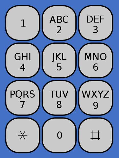
Convert a Phone Number to Strings

The following is a typical phone pad. A number, except for 1 and 0, can be converted to three or four characters. Given a string of digits, we write a backtracking algorithm to convert it to an array of possible strings based on the phone pad convertor. For example, 9 can be converted to W, X, Y, or Z. The output is [“W”, “X”, “Y”, “Z”]. Similarly, the output of 915 is [“WJ”, ”WK”, ”WL”, ”XJ”, ”XK”, ”XL”, ”YJ”, ”YK”, ”YL”, ”ZJ”, ”ZK”, ”ZL”].

Here is the backtracking algorithm to convert a string of digits:

At line 45, it returns immediately with the empty digits. Alternatively, you can put the logic into backtracking itself: Add a check if (list.length > 0) before line 17. Either way works; it is a matter of personal preference.

The algorithm’s time complexity is

The algorithm’s space complexity is O(n).

These are verifying tests:

Well-Formed Parentheses

A well-formed parenthesis has an equal number of opening and closing parentheses. For example, "(())()" is well-formed, but "(((())" is not.

In addition, reading from left to right, the closing parenthesis count cannot exceed the opening parenthesis count. Therefore, "(()))(" is not well-formed.

Here is the algorithm to build the target pairs of well-formed parentheses:

The the total number of valid parentheses strings is the nth Catalan number, which is asymptotically bounded by

The algorithm’s time complexity is

The algorithm’s space complexity is O(n).

These are verifying tests:

Word Search

A word search puzzle is a word game that consists of the letters on a board, which is a rectangular shape. The objective is to find a word hidden inside the board. A word can continue to a consecutive cell in the direction of left, right, up, or down. Each cell can be visited at most once. A word can be a sentence too, i.e., it can include spaces and punctuations.

For example, we can find "it is good!" on the following board.

[['i', 't', ' ', '!'],
 ['a', 'b', 'i', '!'],
 ['g', ' ', 's', '!'],
 ['o', 'o', 'd', '!']]

Here is the backtrack algorithm to search a word:

If the board does not need to be recovered after marking, line 39 can return immediately if the result is true.

Assuming the board is m x n, and the string length is s, the algorithm’s time complexity is

The algorithm’s space complexity is O(1).

These are verifying tests:

Sudoku

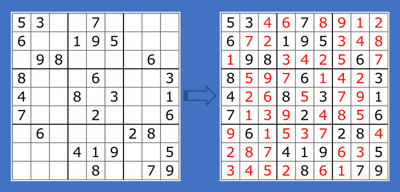
Sudoku is a logic-based, combinatorial number-placement puzzle. The objective is to fill a 9×9 grid with digits so that each column, each row, and each of the nine 3×3 subgrids that compose the grid contain all of the digits from 1 to 9.

The following is an example from Wikipedia.

Here is the backtrack algorithm to fill in Sudoku:

For m unfilled cells, The algorithm’s time complexity is

The algorithm’s space complexity is O(1).

These are verifying tests:

Conclusion

There are many variations of backtracking problems. Practice makes perfect.

The following are other interview guides:

Thanks for reading.

Want to Connect?

If you are interested, check out my directory of web development articles.