The Power of the Exponential

Borne from the notion of self-similar growth, the exponential has far more utility than being just another function.

From pandemics to economics, the exponential growth is a common phrase used to emphasize a dramatic level of change. So how do we understand this notion rigorously?

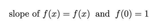
To begin, we consider a function whose growth is proportional to itself. In calculus, this can be defined as a function whose slope is itself. In other words, we are attempting to solve the following equation:

How is all this related to compound interests? It turns out that hidden in this definition is a continuous recursive behavior. Furthermore, the recursion has applications beyond simple growing behavior: we can compound more abstract things, like rotations, translations, and probabilities.

Exponential as Recursions

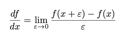
To reveal the continuous recursion, we need to dig deeper to the definition of the slope (or alternatively, the growth) of a function. This is defined as taking the limit of a progressive series of approximations:

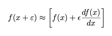
If we ignore the limit symbol, we can better understand what it means when a function’s slope is itself:

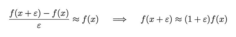
Where we have used the approximate ≈ symbol to indicate approximate behaviors for very small ε. While our discussion is slightly sloppy mathematically, it can be made rigorous using Taylor’s theorem.

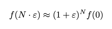
The beauty of this equation is its recursive nature: Say if I want the value of f(1000ε), I just need to multiply f(0) by (1+ε) 1000 times. In other words,

Even though the approximation only works for small ε, N can be very large. In particular, for any x value, we can always choose N large enough so that x = ε ⋅ N, and the above equation applies. This way, we can solve for f(x) recursively:

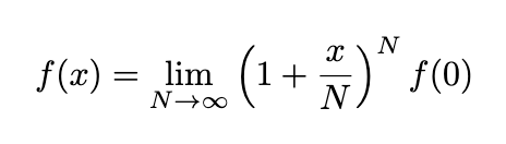
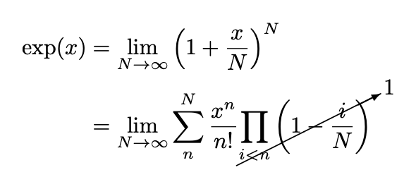
Where we have replace the ≈ sign by =, as we send ε to 0 and the approximation becomes exact. Substituting f(0) = 1 leads to a formula for the exponential function,

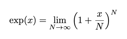
This equation defines the meaning of continuous compounding interest: Say x is an annual interest rate, N = 1 corresponds to once per year interest payment. As we increase to N = 12 (monthly interest), the rate goes down but the payment frequency increases. We can keep increasing N, and the payment frequency would increase to daily, hourly, per minute, per second… etc. The result will ultimately converge to the continuous interest limit — the exponential.

This continuous compounding property is applicable anywhere on the exponential curve. For instance:

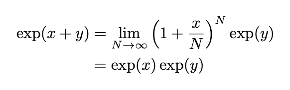
So that compounding will occurs in exactly the same way for any y. This makes sense intuitively: If I’ve been earning interest at a bank for a year, the future interest would be exactly the same as if I deposited the compounded amount I have today.

This also reveals another interesting property: that exponential converts sums into products. This is the reason why the exponential is related to the concept of the exponent: We can define the constant e = exp(1), so that exp(n) can be computed by multiplying e, n times. This justifies writing exp(x) as eˣ.

Product to Series

While the limit definition is intuitive, it is not useful for numerical computations. There is an alternative representation through infinite sums

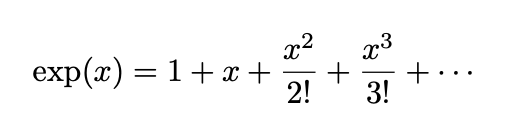
We can understand this sum in multiple ways: First, when computing the derivative term-by-term, we can verify that the series satisfies df/dx = f. Second, this can be directly computed from the compounding formula using Binomial theorem:

In the examples below, we’ll find many useful application of this series representation.

Exponential Applications

It turns out, the concept of continuous compounding doesn’t just apply to the growth of a function. In fact, any general operation that exhibit self-similar behaviors can be rewritten using the exponential form. Below are some examples:

Translation

It is actually possible to use compounding for a general (smooth) function. From the definition of the derivative, we can write

To convert this to a recursive behavior, we need to think of df/dx as an operation (taking the slope of ) ∂ₓ, acting on the function f. This way, we can compound the operation like we compound numbers:

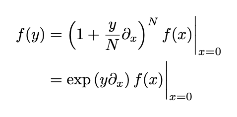
But having an exponential of an operation isn’t all that useful. To make practical sense we need to substitute in the series representation:

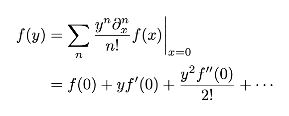
So we’ve just recovered the Taylor’s series! Although the logic might be a bit circular since the initial compounding equation would likely require Taylor’s theorem to be made fully rigorous.

Rotation

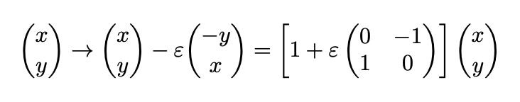
Take any point on a unit circle centered around the origin, say (x, y). We have x² + y² = 1. We can perform a small amount of rotation, say ε, as measured by the arc-length. Using matrix notations, the updated point after the rotation would be:

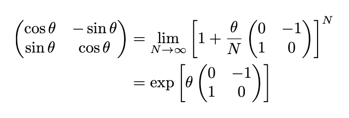
We can compound this tiny rotation in the same way as we compound interest. Say we want to perform a finite rotation θ, measured by the arc-length. We can accomplish this by dividing it into N tiny rotations and compound them. The final result would be the full rotation matrix:

If we use the symbol i to represent the matrix inside the exponential, we find that

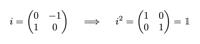
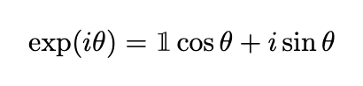
We see that i behaves just like the imaginary number. This way, we have just proved the Euler’s formula

Probability

In this last example, we will derive one of the well-known statistical distributions called the Poisson distribution. This distribution is generated by continuous random events.

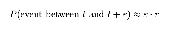
What does that mean? Take bird watching for example, we can model the number of birds we find as a probability distribution. At every small time interval, there is some small probability that I’d see one bird. For small enough time this probability would be proportional to the length of the interval:

Then, if we write the probability of having n events at time t as Pₙ(t). We. can compute an updated probability after a tiny extra amount of time ε has passed:

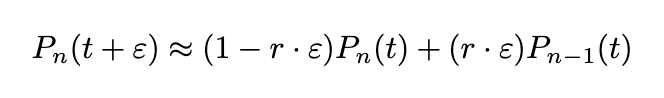
Where the first term captures the loss of probability due to n being incremented. The second term captures the gain of probability coming from an initially smaller n.

Once again, we want to rewrite this in a factorized form to apply compounding. Let’s define an operator Δ to do that

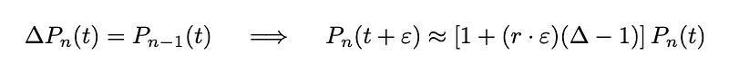
Taking the continuous limit, we get

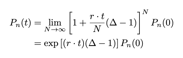
Similar to the case of translation, having exponential of an operation isn’t all that useful. But we can use the series representation

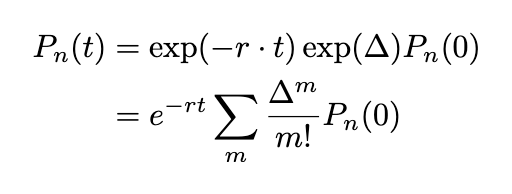
Now, at t = 0, only P₀ is non-zero (we start with no event). So the terms in the series will be zero unless m = n. We can then replace r⋅t by λ and rewrite:

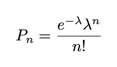
We have just derived Poisson statistics.

Epilogue

To summarize, we see that the exponential can be defined by a self-similar growth. This growth leads to the definition of continuous compounding, which also leads to an infinite series representation.

We then see that this idea can be applied in more general ways, from translation to probability. Our application is by no means exhaustive, as it is just part of the more general concept of Lie Exponential.

Finally, this article showcase a general principle in math and physics: that the power of a formula doesn’t just lie with its specific definition and properties, but rather its generality. Therefore, it is critically important for us to clearly acknowledge assumptions behind every formula and definitions, so that we can utilize the full power of the mathematical machinery. The end result can often lead to un-expected goldmines.

If you find this interesting, you may also enjoy my other mathematical expositions: