Summary

The article discusses the solution to the Gaussian integral using polar coordinates, revealing the integral's surprising result involving π and its connection to the normal distribution curve.

Abstract

The article delves into the Gaussian integral, a well-known integral that cannot be solved using standard integration techniques. The author explains that the integral's indefinite form has no solution in elementary functions and requires the use of the error function. The solution process involves defining the integral as a variable, manipulating it by squaring the integral expression, and converting the resulting double integral into polar coordinates. This approach simplifies the integral, allowing for the application of u-substitution, and ultimately reveals that the integral's value is related to π. The article also connects the integrand to the normal distribution curve, highlighting that the integral represents the area under the curve, which is normalized by dividing by the square root of π to obtain the probability density function of a standard normal distribution.

Opinions

The author finds the Gaussian integral's solution, which involves π, to be fascinating.
The method of solving the integral by converting to polar coordinates is considered creative and interesting.
The connection between the Gaussian integral and the normal distribution curve is seen as a point of interest, emphasizing the real-world application of the integral in probability and statistics.
The author acknowledges that readers familiar with the integral may not find new information but expresses hope that the article will be enlightening for those unfamiliar with the topic.
The fact that the integrand is a normal distribution curve, albeit not normalized, is presented as an intriguing aspect of the integral.

Solving the Gaussian Integral Using Polar Coordinates

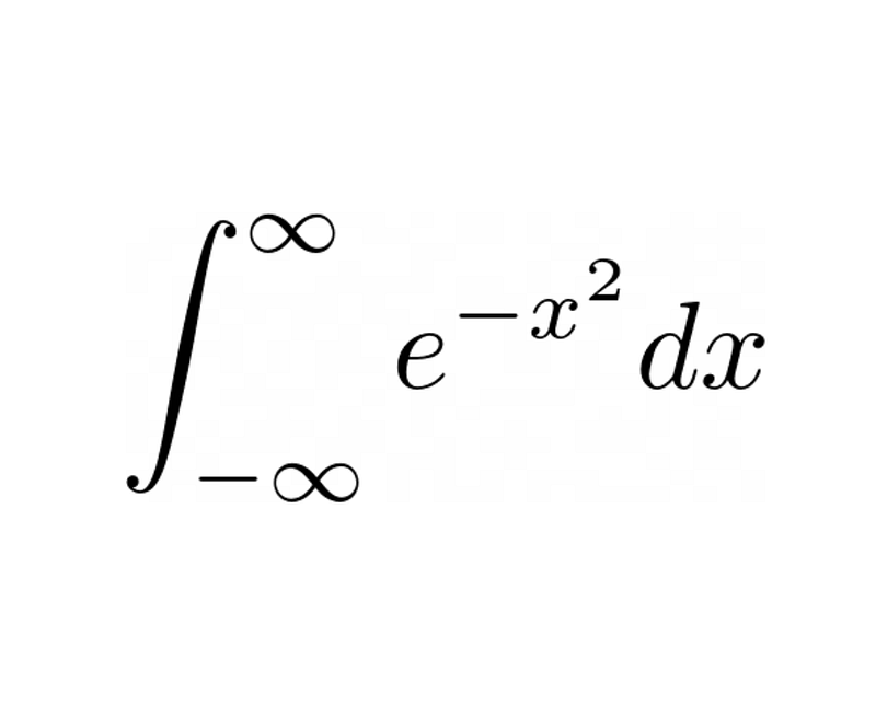
In this article, I will be solving the infamous Gaussian integral shown below that is known for it’s surprising solution and rather creative method of solving. For those who are already familiar with this integral you may not learn much as I will just be going through the standard polar coordinates method, but for those who are not familiar, this may be an interesting article for you.

The Normal Distribution Curve

Before even attempting to solve this, I would like to just focus on the integrand for a second and graph it as it may seem familiar to some people:

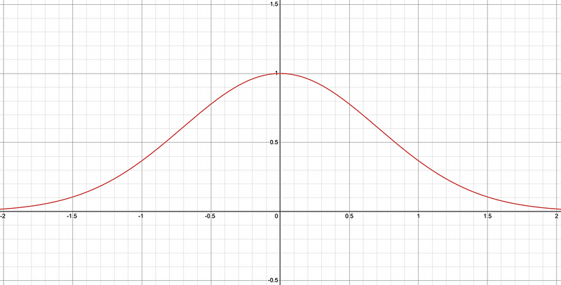
Above is a graph of y = exp(-x²) which may remind you of the normal distribution curve (or bell curve), and that is because it actually is indeed the normal distribution curve, just not normalized so that the area under the curve is 1. The actual area under the curve is precisely what we will be calculating later in this article. In fact, the actual expression for the normal distribution curve is as follows:

Probability density function for a normal distribution

Where μ is the mean and σ is the variance. If you look at this expression carefully you may notice that it does in fact have the exp(-x²) term, and that this is really just exp(-x²) but with horizontal translations (to account for the mean) and stretches (to account for the variance). Although this fact doesn’t neccesarily help us with solving the integral, I find it quite interesitng and I will be returning to it at the end of this article.

Solving the Gaussian Integral

Now, we can attempt to solve the actual integral. To begin, it may already be obvious that while this integral seems simple enough, it cannot actually be solved using standard integration techniques like u-substitution or even integration by parts. In fact, not only can it not be solved using simple integration techniques, the indefinite integral of the Gaussian integral actually has no solution in terms of elementary functions. Instead, a special function known as the error function must be used which is outside the scope of this article. So how exactly do we go about solving this integral if we can’t even solve its indefinite integral? Well, it begins by first defining the Gaussian integral as the letter I (or any other letter) as follows:

What we want to realize here, is that x in this expression is really just a ‘dummy variable’, and so altering the letter we choose for x should not change the actual output value of the integral, I. Hence, the following must be true:

Now, you may be wondering why we are doing this, but it may become clear once we multiply these two integrals and convert it into a double integral:

If it is not obvious why this turns into a double integral, we can first look at the second line where I brought the entire integral with respect to y inside the other integral. This works since that whole integral is essentially just a constant, and constants can be brought inside or outside an integral freely. Furthermore, in the third line I brought the exp(-x²) term inside the second integral which is also valid since a function of x is treated as a constant when integrating with respect to y.

Hence, we end up with the final double integral shown in the fourth line which can be solved by converting to polar coordinates. Now, when making changes of variables it is important to consider how the bounds of integration will change. If we look at the current bounds, we are essentially integrating over all of ℝ² space. To do the same in polar coordinates, we just have to vary our radial coordinate, r, from 0 to ∞ to cover all possible radial distances and our angular coordinate, θ, from 0 to 2π to cover the full 360° rotation. I find this step quite interesting since it essentially makes use of the fact that an infinitely large square would cover the same space as an infinitely large circle.

Finally, we must make sure to not forget the Jacobian of this change of variables which is just r (read more about the Jacobian in this article). Putting all this together, we can finally solve the double integral:

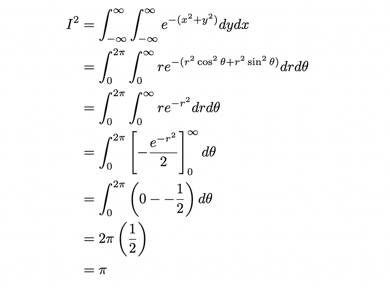
Notice how the extra r term that gets added on from the Jacobian allows for u-substitution to be used in the fourth line, making the integral much easier to solve. Now, if we remember that this final result, π, that we just got is equal to I², we can conclude the following:

Personally, I find the fact the the square root of π is the solution to this integral fascinating, and the way in which we temporarily had to switch to multivariable calculus and use polar coordinates in the process of solving a single variable integral very interesting as well.

Returning to the Normal Distribution Curve

Finally, to end things off, I would like to quickly connect this back to the normal distribution curve I was talking about earlier. If the area under the y = exp(-x²) is the square root of π, all we have to do to normalize it is to divide it by the square root of π to get the following:

Now, if you look back at the expression for the probability density function of a normal distribution curve and let the mean, μ, equal zero and the variance, σ, equal to 1 over the square root of 2, we will end up with the exact same expression as you can confirm below:

Hence, confirming that the integrand of the Gaussian integral is indeed in the form of a normal distribution curve (that isn’t normalized). Thank you for reading.