Summary

The Jacobian determinant is a fundamental concept in multivariable calculus that arises when performing a change of variables in multiple integrals, serving as a scaling factor to account for the transformation of infinitesimal areas or volumes.

Abstract

The Jacobian determinant, named after Carl Gustav Jacob Jacobi, is crucial in multivariable calculus for evaluating multiple integrals after a change of variables. Initially, the author admits to finding the concept challenging but recognizes its importance for future mathematical discussions. The Jacobian is analogous to the derivative in single variable calculus, which scales the differential element during integration. In multivariable contexts, such as double integrals, the Jacobian represents the ratio of the differential area in the new coordinate system to the original one. The derivation of the Jacobian involves expressing an infinitesimal area in terms of the new variables, typically by considering the transformation of vectors in the coordinate change and calculating the area of the resulting parallelogram using the cross product. This process reveals the Jacobian as the determinant of a matrix composed of partial derivatives of the new variables with respect to the old ones. The article concludes with an example of calculating the Jacobian for polar coordinates, confirming that it simplifies to the radial coordinate r.

Opinions

The author initially struggled with understanding the Jacobian but emphasizes its significance in multivariable calculus.
The Jacobian is presented as a multivariable analogue to the derivative in single variable calculus, suggesting a conceptual continuity between the two.
The article suggests that a geometric interpretation of the Jacobian, involving the transformation of infinitesimal areas, is key to understanding its role in integration.
The author believes that the derivation provided, although not rigorous, offers valuable intuition about the nature and utility of the Jacobian determinant.
By demonstrating the calculation of the Jacobian for polar coordinates, the author implies that the concept can be made accessible and practical with the right explanations.

The Jacobian Determinant: How exactly does it work?

The Jacobian… If you are familiar with any multivariable calculus you may have heard of this term. Honestly speaking, the first time I learned about the Jacobian I did not understand how it worked at all, but knowing that the Jacobian is heavily used throughout multivariable calculus and that there will be articles in the future I want to write that use it, in this article, I will finally attempt to give my best explanation of it.

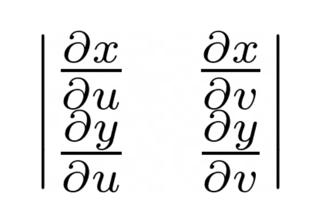
The Jacobian determinant for two variables

Named after German mathematician Carl Gustav Jacob Jacobi, the Jacobian determinant (or just the Jacobian) is required when evaluating multiple integrals after undergoing a change of variables.

To understand the Jacobian, it may help to consider the analogous case in single variable calculus where a change of variable is used. Consider we have the integral of some function f(x), and we wish to undergo the change of variables of x = g(u). Now, using the fact that x = g(u), we can get the following equation:

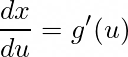
Which if rearranged will give dx = g’(u)du. Substituting this into the original integral, we will get the following:

That extra g’(u) term that must be multiplied to account for scaling is essentially what the Jacobian is but in multivariable calculus. In fact, a double integral undergoing a change of variables will look something like this:

Where J(u,v) is what is known as the Jacobian. However, unlike with g’(u), it is still unclear how to determine how to calculate the Jacobian, so we must derive and expression for it. To do this, we first need to realize the fact that the Jacobian appears when rewriting the infinitesimal area, dydx (or just dA) in terms of du and dv. Therefore, we must somehow express this infinitesimal area, dA, in terms of du and dv.

Deriving the Jacobian

To begin, it might actually help to begin in the uv-coordinate system and then see how an infinitesimal area in terms of du and dv would transform to the xy-coordinate system under the coordinate change. That way we will end up with an infinitesimal area in the xy-coordinate system but in terms of the uv-coordinate system which is precisely what we want.

Hence, we can first consider an infinitesimally small rectangle that has side lengths du and dv. We can express this rectangle in terms of two vectors, (0, dv) and (du, 0) and we can simply observe how these vectors get scaled under the coordinate change to create a new infinitesimal area (usually a parallelogram) in the xy-plane. These two vectors can be seen on the left of the figure below:

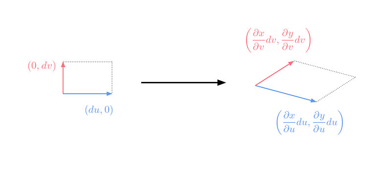
Now, we must figure how how the two vectors get transformed due to the coordinate change. To begin, we can look at the blue vector, (du, 0). Recognizing that the two inputs of a vector in the xy-coordinate system is the x-coordinate and y-coordinate, all we have to do is figure out by how much each x and y coordinate changes due to the infinitesimally small change in u. This can simply be done using partial derivates since the small change in x that occurs due to the small change in u will just be equal to the partial derivative of x with respect to u times du. The same can be done with the y-coordinate and combining the two will give the new blue vector shown on the right in the figure above. Using the exact same method, the transformation the red vector, (0, dv), undergoes can be found to get the new red vector in the xy-plane as shown above.

Now it may be clear why we decided to do this in terms of vectors because the area of the new infinitesimal area we just created can be calculated by using the fact the area of a parallelogram created by two vectors is equal the magnitude of the cross product of those two vectors. Hence, using this fact, our new infinitesimal area can be expressed as the following:

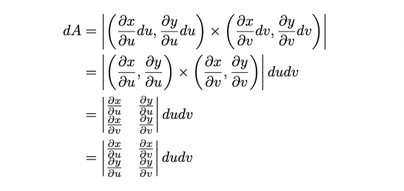
Notice how in the last step I switched two of the partial derivates in the determinant, but this will not actually change the final value as you can confirm. Referring back to the fact that dxdy = dA = J(u, v)dudv, we can recognize that the determinant shown above is this J(u, v) term, also known as the Jacobian. While this derivation is far from rigorous, I hope that it can provide a bit of the intuition of where the Jacobian comes from and what it actually does.

The Jacobian for Polar Coordinates

Now that we know the expression for the Jacobian, I would like to finish with an example calculation for the Jacobian in polar coordinates. For those familiar with multivariable calculus you may already know that this is just r, but we can prove this using the determinant we just derived.

First, we must express x and y in terms of our polar coordinates r and θ. This can be done as follows:

Now, we can calculate the four partial derivatives required to calculate the Jacobian:

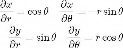
Finally we can substitute these four partial derivatives into the determinant and simplify using the Pythagorean identity as shown below:

Hence, we have just confirmed that the Jacobian for polar coordinates is indeed just r, and this was done using the determinant expression of the Jacobian. While polar coordinates was the example I used, this can work with all other valid coordinate changes, and if we were to work with triple integrals, a similar Jacobian determinant exists that instead has three rows and three columns corresponding to each of the three coordinates in the two coordinate systems.