
The Charged Particle Lagrangian
Everything in Physics can be represented with a Lagrangian, including particles governed by Maxwell’s Equations.
Over the past few articles, I’ve been building up Lagrangian Mechanics as this powerful tool, but I have yet to show that it works for charged particles. More specifically, I have not in any way accounted for magnetism. To deal with magnetism, we need to talk about Maxwell’s Equations.
Everyone and their grandma has written an article or made videos explaining Maxwell’s Equations. I don’t want to duplicate work, so I’m going to proceed with a Lagrangian/Experimentalist approach to electromagnetism.
Check Your Understanding
This article is a little long and mostly consists of derivations, so I’m only asking a few questions.
Deriving the Formula for the Curl
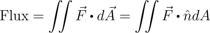
In a previous article, we derived the formula for the divergence from first principles. As a brief summary, we want to measure the total flux out of a 3D box.
We do so using the integral below.
We have six sides for the box that correspond to the left, right, front, back, bottom, and top of the box. To get the total flux, we add them all up.
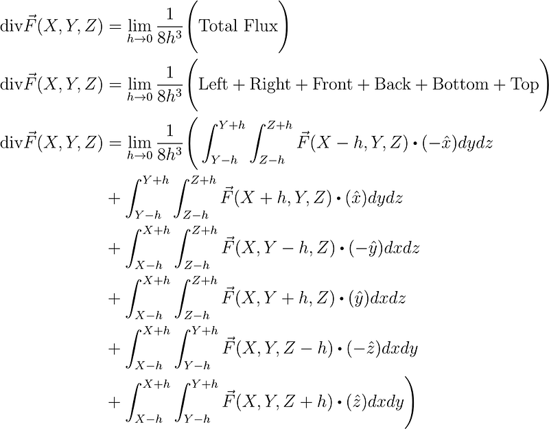
We then get rid of the dot products.
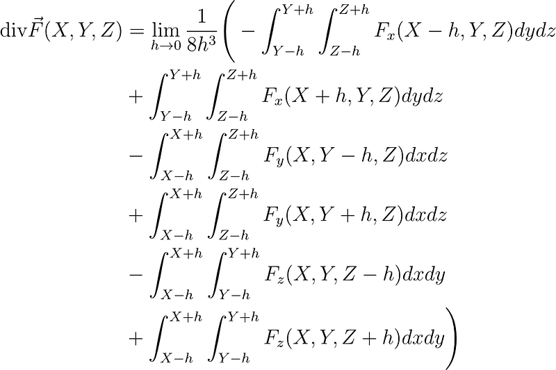
At that point, we use the fact that we’re taking the limit as h goes to zero to argue that all the integrals will converge to the values of the integrand.
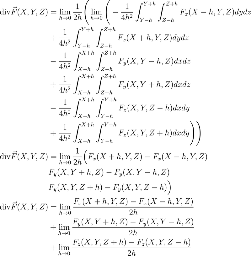
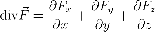
We can then finish the process by rewriting everything in terms of partial derivatives.
Use a similar process to derive the curl. As a hint, you can use a 2D box to account for the rotation.
Find the Proportionality Constant
In this article, we’re going to guess the relationship
Design an experiment to determine the proportionality constant.
Kepler Problem for Charges
Say we have a negative charge orbiting a positive charge. Both the negative and the positive charges are so small that gravity is negligible, but the positive charge is significantly more massive than the negative charge. Use the Lagrangian for a charged particle (or the Lorentz Force Law) along with Maxwell’s Equations to find the equations of motion. If possible, try running a numerical simulation of the particle’s motion. Do stable, bound orbits like a planet orbiting a star exist?
Prerequisites
For this article, all you need to know is
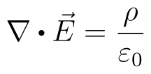
- The divergence of the electric field is proportional to the charge (a.k.a. Gauss’s Law).
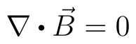
- The divergence of the magnetic field is zero (a.k.a. Gauss’s Law for Magnetism).
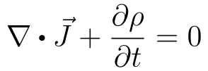
- Charge is conserved. More specifically, charge follows the continuity equation given below.
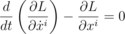
- We can find the equations of motion for any system by creating an object called the Lagrangian and plugging it into the Euler-Lagrange equations.
We derived both Gauss’s Law and Gauss’s Law for Magnetism in a previous article, so we aren’t going to repeat ourselves here. I’ve also discussed continuity equations in one of the exercises of that same article. Furthermore, we’ve derived Lagrangian Mechanics over three articles starting with An Intro to Differential Geometry. You might want to read it to understand why I’m using subscript and superscript letters at various points, why I’m raising and lowering indices, and how the metric tensor relates to the dot product, but I’m going to be converting everything into Cartesian coordinates for most of the derivation. You might also want to brush up on your Vector Calculus, but I’ll be introducing every new identity required in this article.
Related Reading
Electromagnetism is a vast field, and I do not want to cover it all. For this reason, I’m going to recommend a few standard textbooks.
- Introduction to Electrodynamics by David J. Griffiths is the standard undergrad textbook in the field.
- Electricity and Magnetism by Edward M. Purcell directly incorporates Special Relativity into Electromagnetism and has some tricky problems to cut your teeth on.
- Classical Electrodynamics by John David Jackson strikes fear into the hearts of physicists. It covers a lot of what Griffith’s textbook covers, but in much greater depth with much more rigor.
Unfortunately, I don’t have as many online resources as I normally do because no one wants to cover the boring parts of Physics.
WARNING: Do Not Connect a Potential Difference Without a Load
I’m going to talk about several experiments that you could perform at home. For example, to test Ampère’s Law, you could send a current through two wires and check how they bend or you could use a moving magnetic field to generate current in line with Faraday’s Law of Induction. In any case, you should never connect a potential difference without a load unless you’re an electrician or you’re several meters away. Doing so would create a short circuit that could end up delivering a lot of energy somewhere you don’t want it to go, which could lead to an explosion.
What If I’m a Trained Electrician or If I’ve Done the Math or If I Have a Working Version or…?
Good for you, but if I don’t have this disclaimer in the article, someone is going to do the equivalent of sticking a fork in an electric socket.
Assumptions
While I normally take a historical approach, the history of electromagnetism gets a little too messy to follow without effort. It feels like every scientist between Coulomb and Maxwell chose a few random sections of a modern electromagnetism textbook to discover, but with a lot of baggage like the electric and magnetic fluids and older math. For this reason, I’m going to take two facts as assumptions for the model:
- Matter is made up of charged particles.
- The motion of these particles is current.
Ampère’s Force Law
Ampère did experiments on the force per unit length of two parallel current-carrying wires and found the relation known as Ampère’s Force Law.
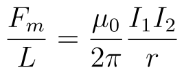
In other words, the force per unit length one current-carrying wire exerts on another current-carrying wire is proportional to the currents in both wires and inversely proportional to the distance between the two wires. The direction also matters in that currents flowing in the same direction repel while currents flowing in the opposite direction attract. We’re going to take it as a given empirical fact about the world and come up with a theoretical background for it.
Observations
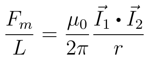
Ampère’s Force Law only depends on the distance between the two straight, parallel wires and not the orientation in space or the distance along the wire. The force field around a straight wire with a constant current must therefore have cylindrical symmetry, i.e. F(ρ, φ, z) = F(ρ). The relative orientation of the two wires determines the magnitude of the force. As with many cases in Physics, we can measure this relative magnitude with a dot product.
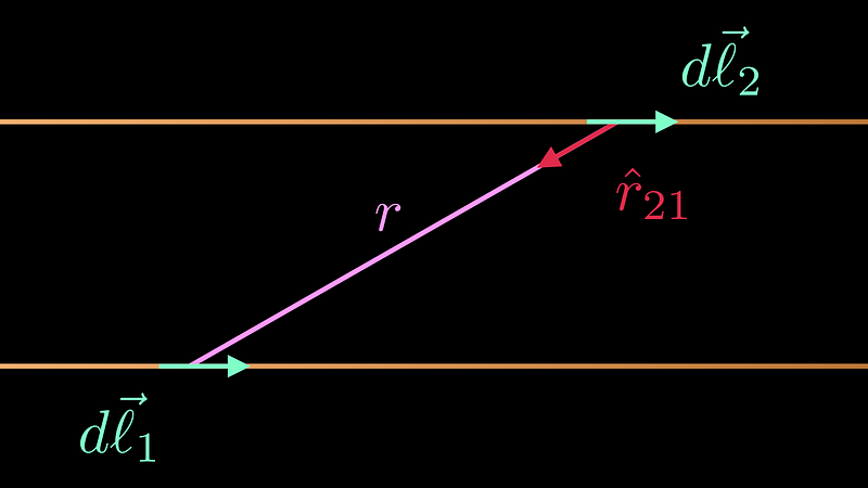
We have to be careful, though, because if the distance between the two wires is not constant, different parts of the wire could experience different forces. To fix that fact, we can turn everything into an integral over both wires. Since we have cylindrical symmetry and F ∝1/r, the integrand will be proportional to 1/r².
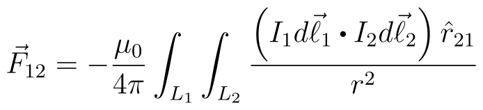
- The term inside the parentheses is the differential form of the I₁ ⋅ I₂.
- dℓ₁ and dℓ₂ represent small segments of the first and second wire.
- I₁ and I₂ represent the currents flowing through the small segments of each wire.
- The L₁ and L₂ terms represent the lengths of the wire as intervals.
- The hat r₂₁ term represents the unit vector pointing from dℓ₂ and dℓ₁.
- r represents the distance between dℓ₁ and dℓ₂.
Why Does this Force Exist?
Here’s where I have to bring in my assumptions. Since matter is made up of charged particles whose movement is current, moving charged particles must exert a force on each other. Up to this point, we’ve only discussed two forces that could affect a charged particle: gravity and the electrostatic force. Neither depends on the velocity of the charged particles.
The Electrostatic Approach
If the laws of physics are the same in every inertial reference frame, you could convert the force between the two wires into an electrostatic force by moving to the reference frame of a moving charged particle in one of the wires. In that frame, the charge isn’t moving so it exerts an electrostatic force on the charges in the other wire. We can measure the force per charge using the electric field.
The force between two charged objects depends on the charge density of both objects. For you to claim that there is an electrostatic force between the two wires in this frame, you have to argue that moving to the charged particle frame somehow changes the charge density of the wires.
We haven’t talked about Special Relativity yet, so we’re not going to solve the problem this way. If you’re really interested in this approach, check out Purcell’s textbook. Instead, we’re going to take a Lagrangian approach to the problem.
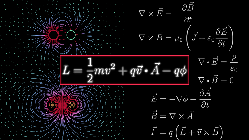
The Lagrangian for a Classical Charged Particle
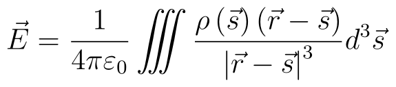
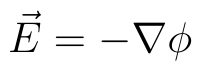
In previous articles, we’ve established that the electrostatic force can be described as the gradient of some scalar function we call the electric potential.
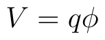
Since the electric potential is related to the potential energy by the equation
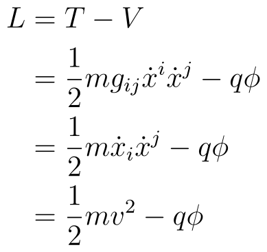
We can write the electrostatic (i.e. ignoring forces from any moving charges) Lagrangian as
Electrostatics is still valid, but we need to add another force to the equation to account for Ampère’s Force Law. This force has to depend on
- all the nearby currents,
- the magnitude of the charge,
- the direction of the velocity relative to the nearby currents,
- and the magnitude of the velocity.
So here’s the plan. We’re going to combine all the effects of all the nearby currents into one field. This field cannot be a scalar field since it needs some directional information, so we’ll make it a vector field. We’ll call this vector field the magnetic vector potential for reasons we’ll discuss later and denote with an A. To add in the magnitude of the charge, we’re going to multiply this field by the charge. Lastly, we use dot products to find relative directions, so we’re going to guess that the term is going to be proportional to the dot product of the velocity and the vector field. Since the dot product already includes the magnitude information, we don’t need to do anything special to include the magnitude of the velocity. Putting it all together gives us this guess for the Lagrangian.
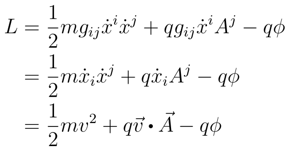
It turns out that this is exactly the right answer, so we just need to connect it to Ampère’s Force Law.
Velocity-Dependent Potentials?
In my earlier derivation of Lagrangian Mechanics, I explicitly assumed that the non-kinetic energy part of the Lagrangian did not depend on the velocity.
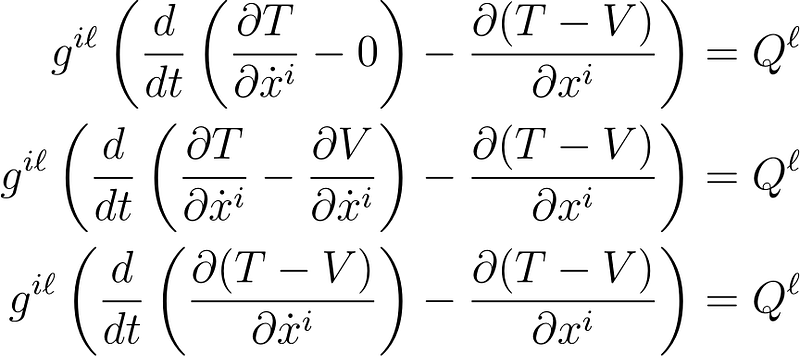
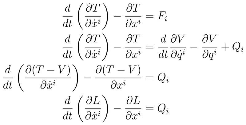
This omission is not a problem since I can expand my definition of a potential to include all forces that can be written in the form
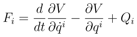
At this point, the derivation becomes
Plugging this Lagrangian into the Euler-Lagrange Equations
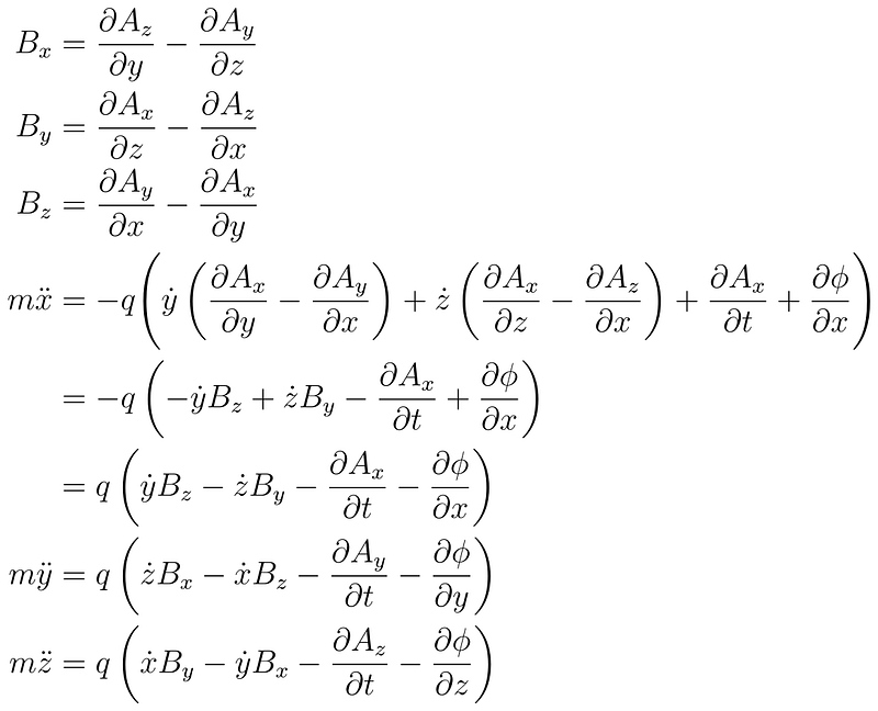
We’ve only added a single term, but A depends on both the position and time and it’s connected to velocity terms. To plug it into the Euler-Lagrange equations, I’m going to need to take a lot of derivatives. Since I don’t want to be here all day, I’m going to do the derivation in Cartesian coordinates instead of generalized coordinates. First, we need to find the necessary derivatives.
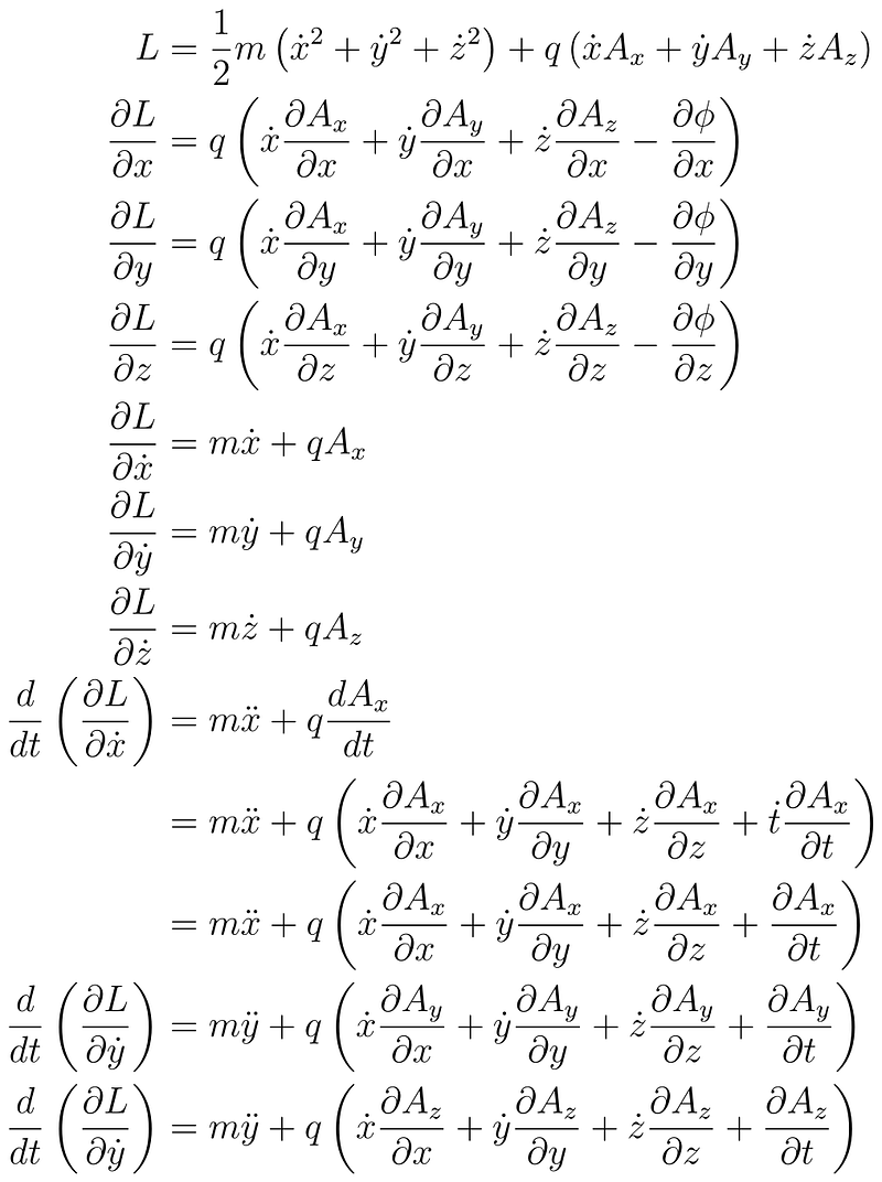
Then, we can plug everything into the Euler-Lagrange equations.
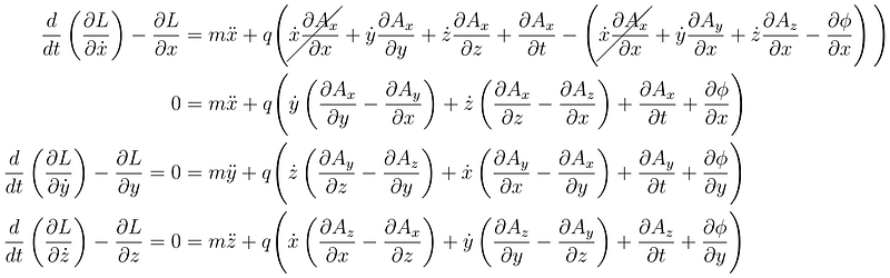
This is quite a mess, but there are a few simplifications we can make.
The Curl
First, we’re going to introduce a concept known as the curl. The curl takes in a vector field that usually represents some kind of velocity field of a fluid flow like the one below

and spits out a vector field that usually represents the angular velocity that an infinitesimal object would experience.
The angular velocity and curl point in the same direction and the magnitude of the curl is twice the angular speed.
I’m going to leave the derivation as an exercise for you. At the end, you should get
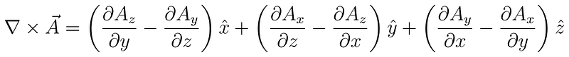
If you go back to the equations of motion we’ve derived, you should be able to see that we can represent all the partial derivatives in the velocity part of the force as components of a curl of A. To clean up our notation, we’re going to make a new field out of the curl of A which we’ll call the magnetic field and denote with a B. In other words, B = ∇ × A. With this new field, we can rewrite the equations of motion as
Gauss’s Law for Magnetism
There are a million ways to prove it, but the divergence of a curl is always zero. We can use this definition to conclude that
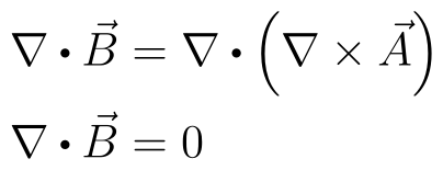
In other words, we get Gauss’s Law for Magnetism by defining the magnetic field in terms of a vector potential.
The Cross Product
If you ever have
- vectors
- in three dimensions
- that are perpendicular to some other vectors
- and have the difference of cross terms,
you’re probably looking at a cross-product. The cross-product is defined as

in Cartesian coordinates according to the right-hand rule (a left-hand rule would flip some signs). If we look back at our equations of motion, we can see that we should be able to write the velocity terms as a cross-product.
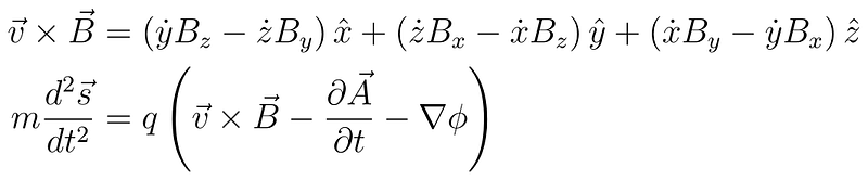
That takes care of almost everything. We just have to deal with the last two terms.
Faraday’s Law of Induction
To deal with the remaining terms properly, we need to talk about Faraday’s Law of Induction. Let’s start with a simple circuit powered by some potential difference. When we connect the two ends of the potential difference with a wire, the charge is free to flow and it starts flowing from one end to the other. If we can detect this flow (say with a light bulb), we can detect potential differences.
So What’s The Problem?
Connect the terminals of a light bulb together with a wire, but no battery. Then, move a magnet back and forth through the closed loop. The light will turn on as you move the magnet and off when the magnet stops moving.
So there must be some potential difference between the two terminals of the light bulb, right? Nope. If that were true, then it would be as if we connected a battery to both terminals. Most of the current would flow through the wire, not the light bulb, which we’d call a short circuit. Furthermore, the current would flow away from one of the terminals and into the other terminals. Instead, you’ll observe that the entire circuit has the same current flowing in the same direction.
To make matters more complicated, moving the magnet only works if we have a closed circuit, but we can create a potential difference in an open circuit. In short, there are far too many problems for us to assume some kind of potential difference.
The Problem
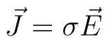
Earlier, when I said that our circuit detected potential differences, I was being inaccurate. Our circuit detects the current, which is determined by the electric field in the wire according to Ohm’s Law (in this case).
Using this definition, we can see that we have an electric field that seems to form a closed loop.
How to Solve the Problem
One way to generate a noticeable electric field in a wire is to create a potential difference between its endpoints, but it seems that we can also generate a noticeable electric field in a closed loop by creating a changing magnetic field. We can represent the first part with the gradient of the electric potential, but the second part of the electric field can’t be represented by the gradient of any field. Gradient forces can only push things downhill from a higher potential to a lower potential, but our potential would have to look like an M.C. Escher painting to achieve a constant force in a loop.
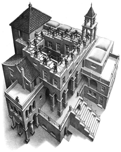
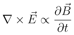
While possible in art, it is impossible for a mathematical object. We need to add something that allows us to make our electric field form closed loops and incorporate a changing magnetic field. Speaking of the magnetic field, we know that it always forms closed loops and it’s defined in terms of a curl, so maybe we should do something with the curl of the electric field. Furthermore, we can take the simplest guess for the relationship and say that the curl is proportional to the partial derivative of the magnetic field with respect to time.
It turns out that this equation is correct if we figure out the proportionality constant.
Lenz’s Law
To figure out the exact constant, you would have to do some experiments where you know how much the magnetic field is changing and the resulting electric field. There are a few ways to figure it out, but all experiments work by measuring the current through a loop of wire as you move a magnet with a known magnetic field around the wire. In either case, you’ll want to use Stokes’ Theorem to simplify your calculation since flux and EMFs are easier to deal with.
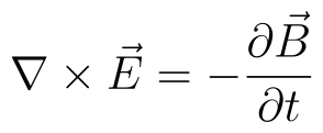
Regardless of the experiment you do, you’ll find the proportionality constant to be -1. Conceptually, the charges move in such a way as to resist the change in the magnetic field, which is known as Lenz’s Law. Using this information, we end up with the Maxwell-Faraday Law.
The New Electric Field
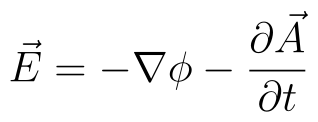
In previous articles, we defined the electric field as
From this article onward, we extend the definition to include the partial time derivative of the vector potential.
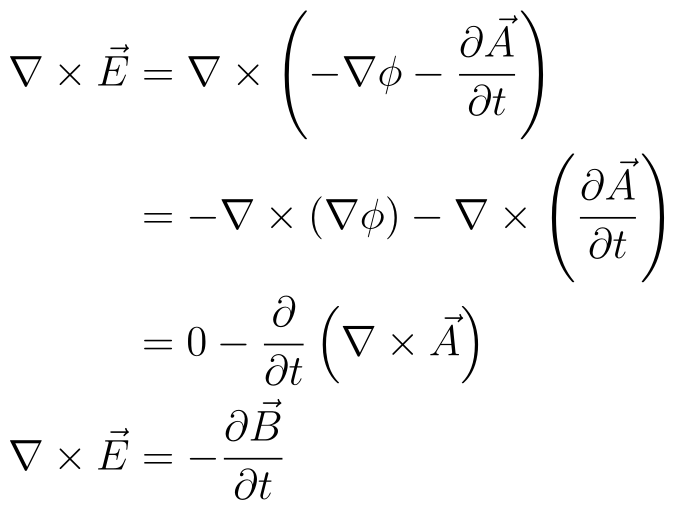
If we then take the curl of this electric field, we end up with the Maxwell-Faraday equation, so everything is consistent.
The Lorentz Force Law
If we plug the new definition of the electric field back into the equations of motion, we get the Lorentz Force Law.
The Ampère-Maxwell Law
So far, we’ve derived several equations governing electromagnetism, but we still need to figure out the relationship between A, B, and the current density J.
Magnetostatics
We’re going to be assuming our system is magnetostatic for a while, which means that all the currents are steady. Note that charges can still move in magnetostatic systems as long as the way they move doesn’t change. To ensure steady currents, we assume that the charge doesn’t build up anywhere. Mathematically, this assumption means that we have a constant charge density.
The magnetostatic assumption allows us to make a few simplifications. First and foremost, we can ignore any relativistic effects and gauge theory, which allows us to derive the Biot-Savart Law instead of the more general Jefimenko’s Equations. Furthermore, by the continuity equation for charge and our assumption of constant charge density, the divergence of the current density is zero.
We’ll be using this fact later to derive Ampère’s Circuital Law, a precursor to the Maxwell-Ampère Law.
Comparing Terms
Ampère’s Force Law currently gives us a relationship between the force between two wires and the Lorentz Force Law gives us the relationship between force, the velocity of charge, and the magnetic field. Our previous approach to Ampère’s Force Law only uses dot products so we’re going to redo our approach by using cross-products.
Finding the Direction of the Magnetic Field
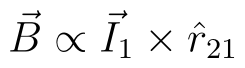
The force is the cross-product of the velocity of the charged particles and the magnetic field. We can use this fact to figure out the direction of the magnetic field. Since the force points from the first wire to the second wire and the velocity points along the wire, the magnetic field needs to curl around the first wire.
Since the magnetic field should be perpendicular to both the current and the direction between the wires, we would expect the magnetic field to be proportional to the cross-product of the current and the direction between them.
Finding the Strength of the Magnetic Field
To figure out the strength, we’re going to use Ampère’s Force Law and the Lorentz Force Law to calculate the force separately, and then compare terms.
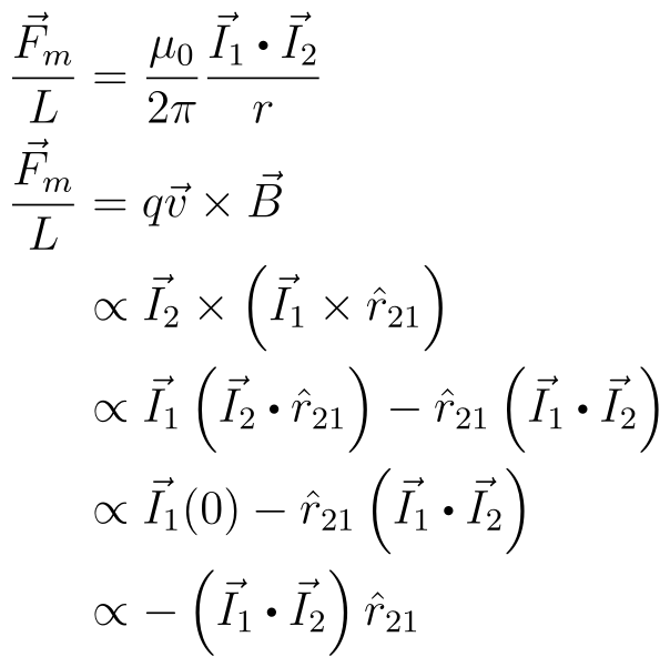
For the two results to be equal, we have to scale the magnetic field by the value –μ₀ / (2 π r). In doing so, we get
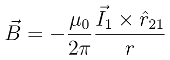
We can get rid of the minus sign by replacing r₂₁ with r₁₂.
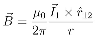
The General Case
While this is fine for one wire, what about multiple wires? What if the current isn’t flowing through an infinite wire? What if the current is flowing through a thick wire? To fix this problem, we can convert everything into an integral. Since we only care about the magnetic field and not the presence of the second wire, we’re going to replace r₁₂ with r – s, where r is the point at which we want to know the field and s is the source of the current we’re looking at. We again had cylindrical symmetry with a 1/r dependence in the special case of one wire, so we’re probably going to have a 1/r² dependence in the integral. Putting everything together gives us
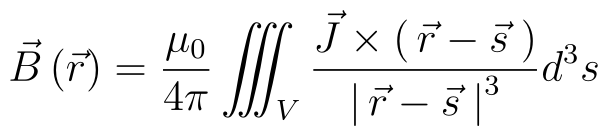
This law is known as the Biot-Savart Law. Since we derived this law assuming magnetostatics, it only works within magnetostatic equations.
The Semi-General Case
If your current is constrained to a wire of arbitrary shape, then the Biot-Savart Law becomes
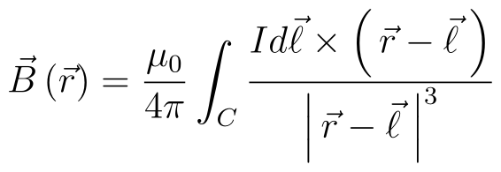
If you have multiple wires, then you can add up multiple contributions from each wire.
The Magnetic Vector Potential in Terms of Currents
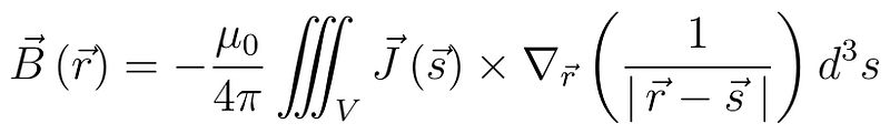
We can also use the Biot-Savart Law to come up with an expression for the vector potential in terms of currents (under the assumption of magnetostatics). To do so, we have to notice that
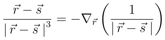
This fact may seem to come out of the blue, but we’ve already derived it when we first introduced potentials. It’s the 3D version of
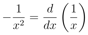
Plugging this fact into the integral gives us
So now, we should look for some identity from Vector Calculus that can help us here. If you go through the entire Wikipedia page or have a lot of free time on your hands, you can find this vector identity
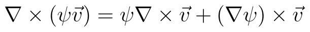
One of the terms has a vector field cross a gradient. Solving for that term gives us

We can then plug this identity into the integral to give us
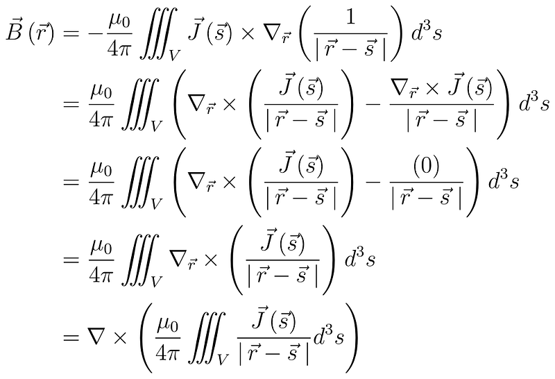
Since B = ∇ × A, we have
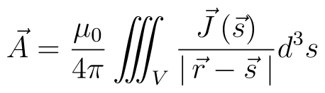
I want to reiterate that this expression only works for magnetostatics, but there is a closely related expression that does work in all cases. We’ll cover it in a later article.
The Ampère Circuital Law
We’re almost done, but there’s one more missing piece. By a corollary of the Helmholtz Decomposition Theorem, we can completely describe a smooth vector field if we know its divergence and curl. Right now, we know the divergence and curl of the electric field, but we only know the divergence of the magnetic field. If we wanted to only talk about electric and magnetic fields, we would need to know the curl of the magnetic field. We currently have an expression for the magnetic field assuming magnetostatics, so let’s take its curl.
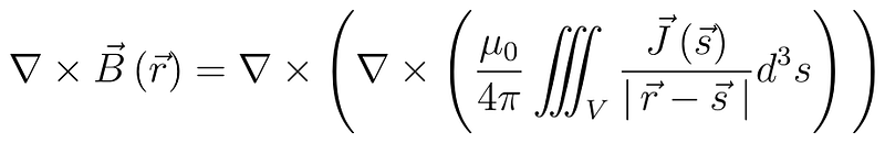
Looking through the table of vector identities gives us the formula for the curl of the curl of a function.
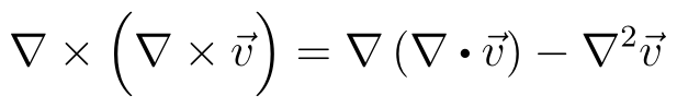
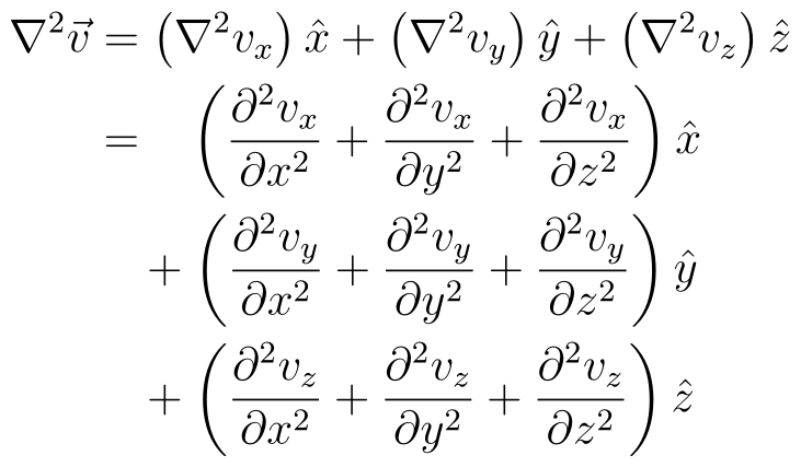
∇² in this case is the vector Laplacian, which is just the Laplacian applied to each component of the vector separately (at least in Cartesian coordinates).
Using this formula, we have
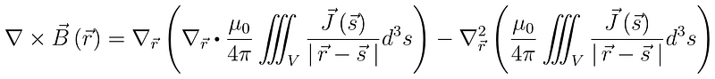
To deal with the first integral, we’re going to move the divergence operator around until we get the divergence of the current density, which we can then set to zero. We can use another identity from Vector Calculus to simplify the first integral.
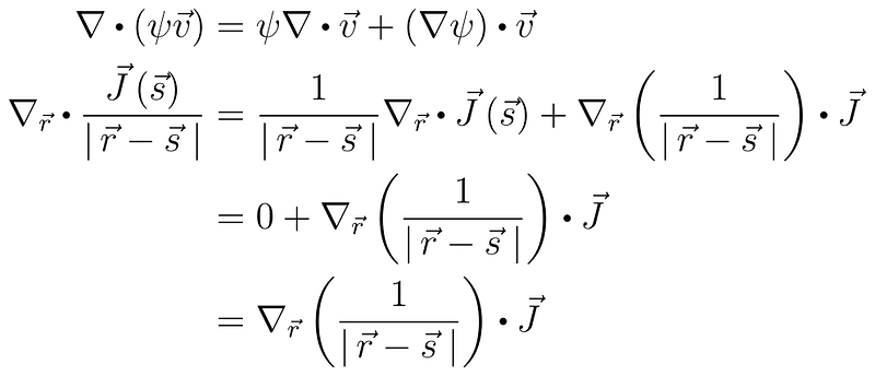
For the second, we can just move the vector Laplacian into the integral, at which point it becomes the normal Laplacian. Applying both of these facts to our equation gives us

We then have two identities that we can use.
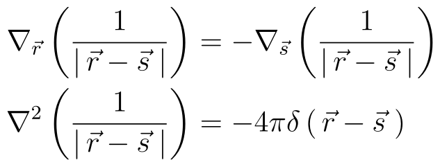
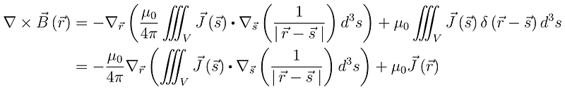
The first comes from the symmetry between r and s. The second is something we derived in the first part of the Dirac Delta article. It just says that the potential from a point source modeled by a Dirac Delta function is proportional to 1/r. Using these identities gives us
To do the remaining integral, we have to use the divergence identity from Vector Calculus that we used earlier, the magnetostatic assumption that the divergence of current is zero, and the divergence theorem.
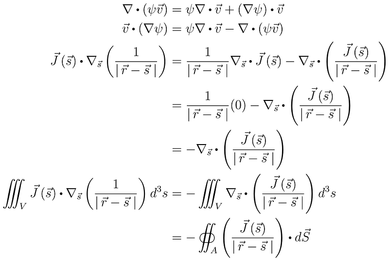
To deal with this final integral, note that we can always define our volumes to completely contain the currents, which means there is no current flowing through the surface, which means the integral is zero.
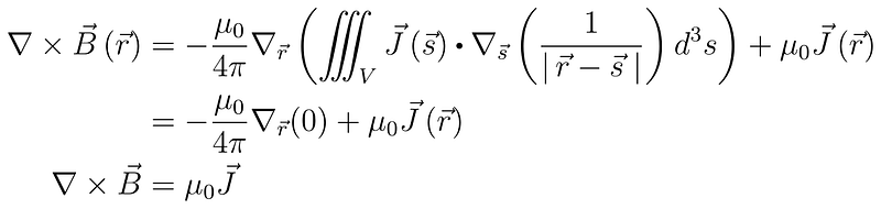
In the end, we get Ampère’s Circuital Law.
Maxwell’s Correction
We still have a problem. We know that charge is conserved, which means it must follow a continuity equation.
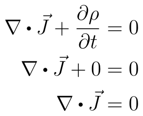
From our current version of Ampère’s Law, we would have
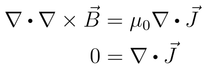
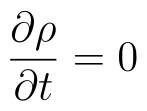
which is only correct under magnetostatic assumptions (i.e. ∂ρ/∂t = ∇⋅J = 0). To fix this problem, we need to add a term whose divergence is equal to the partial derivative of the charge density with respect to time. Our only equation that relates charge density with any kind of divergence is Gauss’s Law, but we can take the time derivative of both sides of the equation and solve for the time derivative of the charge density.
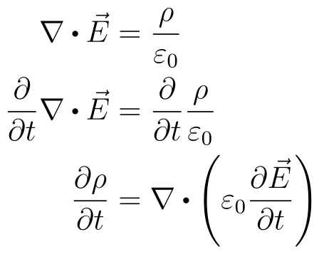
Now, we can plug everything in and get the completed set of equations.
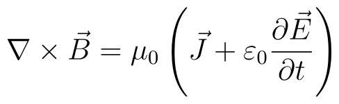
The term we added to Ampère’s Law is known as Maxwell’s Correction or the displacement current.
The Important Equations
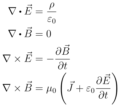
We finally have a complete description of electromagnetism. First, we have Maxwell’s Equations.
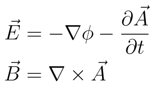
Then, we have the relationships between the potentials and the fields.
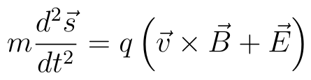
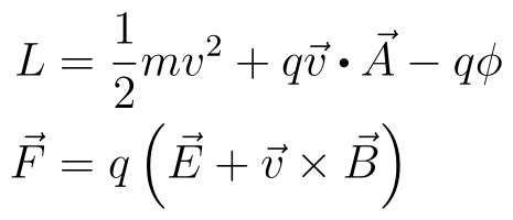
Lastly, we have the equations of motion for a charged particle, which can be given in terms of a Lagrangian or the Lorentz Force Law.
What’s Next?
As I’ve said before, we should be able to write a Lagrangian for pretty much all the major phenomena in Physics. In this article, we showed that we could write a Lagrangian that would give us the correct equations of motion for a charged particle experiencing an electromagnetic force. We’ve looked at Lagrangians for particles, waves, and light, but could there be a Lagrangian for the electromagnetic field? Over the next few articles, we’ll derive a complete theoretical approach to Classical Electromagnetism. I’m still working on them, but I think they’ll cover
- Tangent and Cotangent Spaces, Differential Forms, the Generalized Stokes’ Theorem, Maxwell’s Equations in their integral form (I might split this article into two parts.),
- Lagrangian Field Theory,
- Electromagnetic Optics,
- and Special Relativity
in that order. If you have any questions about any of these topics, let me know and I’ll try to answer them in the corresponding article.
Self-Promotion
If you liked this article, you probably know someone else who will. It would help me out if you could share this article with them. If you really liked this article or any of my other articles, you can help me write them by donating to my ko-fi account. If you’re not already a Medium member and you like the articles on the website, you can name me as your referred member and a portion of your monthly fee will help support me.


