Take Your Forecasting to the Next Level with Harmonic Regression

Unveiling the fascinating relationship between Fourier Series and Time Series

Background & Problem

When we want to model seasonality in our time series we often turn to the SARIMA model. This adds seasonality components to the ARIMA model by finding autoregressors and moving-averages at certain specific lag indexes. For example, monthly data with yearly seasonality will fit autoregressors and moving averages at multiples of 12. You can read more about this process in my previous article here:

However, what if we have daily data with a yearly seasonality of 365.25 days? Or even weekly data with a seasonality of 52.14?

Unfortunately, SARIMA can’t handle this as it is non-integer and also struggles computationally due to the memory required to find patterns in 365 data points each season.

So, what do we do?

Income Fourier series to save the day!

What Is Fourier Series?

Intuition

Fourier series is one of the most interesting discoveries in mathematics which states that:

Any periodic function can be decomposed into a sum of sine and cosine waves

This is a very simple statement but its implications are very significant.

For example, shown below are the functions sin(2x) and cos(3x) and their corresponding summation:

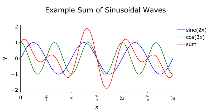
Notice that the functions of sin(2x) and cos(3x) are very uniform and simple functions yet their summation (red line) leads to a more complex pattern. This is the main idea behind the Fourier series.

We can even use the Fourier series to construct a square wave by summing sine waves (harmonics) of different odd number frequencies and amplitudes:

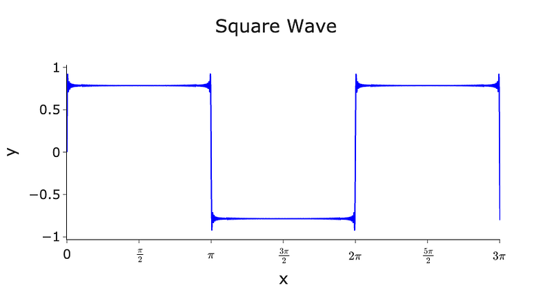
What’s staggering about this result is that we have generated a sharp and straight line plot from smooth sine functions. This shows the true power of the Fourier series to construct any periodic function.

The code used to make these plots is available on my GitHub here:

Theory

As we said above, the Fourier series states that any periodic function can be broken down into a sum of sine and cosine waves. Mathematically, this is written as:

Where:

• A_0: average value of the given periodic function
• A_n: coefficients of the cosine components
• B_n: coefficients of the sine components
• n: the order which is the frequency of the sine or cosine wave, this is referred to as the ‘harmonics’
• P: period of the function

The period, P, and order, n, are known ahead of time. However, the coefficients (A_0, A_n, B_n) need to be calculated to determine which sine and cosine components combined produce the given periodic function. These are normally deduced through integration (see here for an example of this), but luckily most Python data science packages do this process for us!

Link to Forecasting

Are you wondering how does the Fourier series fit into time series forecasting? Well, remember that Fourier series deal with periodic functions and we often find that time series contain some periodic structure (typically seasonality). Therefore, we can use the Fourier series to model any complex seasonal pattern in our time series data!

Pros of using the Fourier series to model seasonality are:

• Any season length
• Model multiple seasonal patterns
• The sensitivity of the Fourier seasonality can be tuned through the order and amplitudes of the sine and cosine components
• Computationally efficient when seasonal periods are greater than ~200

Many of these advantges cannot be achieved with the SARIMA model as it only accepts integer seasonality, a single season, and often runs out of memory when the seasonal period is more than ~200.

Cons of using the Fourier series to model seasonality are:

• Assumes seasonal patterns and cycles remain fixed

The question now begs, how do we add it to our model?

ARIMAX & Exogenous Features

Intuition

For ARIMA models we can add extra external features to aid in the forecasting. These features are called exogenous features and make the ARIMA model become an ARIMAX model. For example, we may use the current interest rates as an exogenous feature when forecasting the value of a house.

You can think of the ARIMAX model as just like regular linear regression with the addition of autoregressors and moving-average components (endogenous variables). The trick here is to allow the Fourier series to be one of these exogenous features or an explanatory variable as is often described in linear regression.

As we are dealing with time series, the exogenous features need to be time indexed just like the autoregressors and moving-averages. They also need to be known at the point of the forecast. For example, if we want to forecast the value of a house in May, we need to know what the interest rates are in May if we want them as an exogenous feature.

Theory

Mathematically, the exogenous features are added to the classic ARIMA model in the following way:

• y: time-series/lags at different time steps
• x: exogenous feature
• β: coefficient for exogenous feature
• ϕ: coefficients of the autoregressive components (lags)
• p: number of autoregressive components
• ε: forecast error terms, the moving-average components
• θ: coefficients of the lagged forecast errors
• q: number of lagged error components

Fourier Series Features

To add the Fourier series as exogenous to an ARIMA model is relatively simple as the coefficients/amplitudes, β, are deduced for us and all we need to provide are the corresponding sine and cosine terms. In pseudo-code, this is equivalent to:

# Sine component
sin(2*pi*frequency*time_index/period)

# Cosine component
cos(2*pi*frequency*time_index/period)

As an example, let’s say we have monthly data with a yearly seasonality and we want the Fourier components for May. This, in pseudo-code, would be:

# Sine component
sin(2*pi*frequency*5/12)

# Cosine component
cos(2*pi*frequency*5/12)

May is the 5th month and there are 12 months in a year.

However, we still have the frequency (the order) value to deduce. This is typically found by passing numerous sine and cosine component orders and letting the model find the most useful ones. In the Python example below we will illustrate this process.

Python Implementation

We will now use harmonic regression and ARIMAX to carry out some real-world forecasting! We will use the US airline passenger dataset from Kaggle.

Data from Kaggle with a CC0 licence.

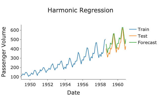
As we can see, the Fourier orders have captured the seasonality quite nicely!

Note: in the above code we used the Box-Cox transform to make the variance stationary. You can learn more about that process here.

Summary and Thoughts

When the seasonality of your time series is a non-integer, has numerous patterns, or is very long (>50 points) then it is preferable to use the Fourier series to model this seasonality component. This can be achieved by adding the Fourier series as an exogenous feature to a regular ARIMA model to make it an ARIMAX. These exogenous features are external covariates that aid in the forecasting of the time series.

The full code can be found at my GitHub here:

Another Thing!

I have a free newsletter, Dishing the Data, where I share weekly tips for becoming a better Data Scientist, and the latest AI news to keep you in the loop. There is no “fluff” or “clickbait”, just pure actionable insights from a practicing Data Scientist.

References and Further Reading

• Forecasting: Principles and Practice: https://otexts.com/fpp2/

Connect With Me!

• YouTube 🎬
• Newsletter 📄
• LinkedIn 👔
• Twitter 🖊
• GitHub 🖥
• Kaggle 🏅

(All emojis designed by OpenMoji — the open-source emoji and icon project. License: CC BY-SA 4.0)