T-distributed Stochastic Neighbor Embedding(t-SNE)

Learn the basics of t-SNE, how it is different than PCA and how to apply t- SNE on MNIST dataset

In this article, you will learn:

• Difference between t-SNE and PCA(Principal Component Analysis)
• Simple to understand explanation of how t-SNE works
• Understand different parameters available for t-SNE
• Applying t-SNE and PCA on MNIST

What if you have hundreds of features or data points in a dataset, and you want to represent them in a 2-dimensional or 3-dimensional space?

Two common techniques to reduce the dimensionality of a dataset while preserving the most information in the dataset are

• Principal Component Analysis(PCA)
• t-Distributed Stochastic Neighbour Embedding(t-SNE)

Goals for reducing the dimensionality of the data

• Preserve as much significant structure or information of the data present in the high-dimensional data as possible in the low-dimensional representation.
• Increase the interpretability of the data in the lower dimension
• Minimizing information loss of data due to dimensionality reduction

What are PCA and t-SNE, and what is the difference or similarity between the two?

Both PCA and t-SNE are unsupervised dimensionality reduction techniques. Both techniques used to visualize the high dimensional data to a lower-dimensional space.

Principal Component Analysis(PCA)

• An unsupervised, deterministic algorithm used for feature extraction as well as visualization
• Applies a linear dimensionality reduction technique where the focus is on keeping the dissimilar points far apart in a lower-dimensional space.
• Transforms the original data to a new data by preserving the variance in the data using eigenvalues.
• Outliers impact PCA.

t-Distributed Stochastic Neighbourh Embedding(t-SNE)

• An unsupervised, randomized algorithm, used only for visualization
• Applies a non-linear dimensionality reduction technique where the focus is on keeping the very similar data points close together in lower-dimensional space.
• Preserves the local structure of the data using student t-distribution to compute the similarity between two points in lower-dimensional space.
• t-SNE uses a heavy-tailed Student-t distribution to compute the similarity between two points in the low-dimensional space rather than a Gaussian distribution, which helps to address the crowding and optimization problems.
• Outliers do not impact t-SNE

T-distributed Stochastic Neighbor Embedding (t-SNE) is an unsupervised machine learning algorithm for visualization developed by Laurens van der Maaten and Geoffrey Hinton.

How does t-SNE work?

Step 1: Find the pairwise similarity between nearby points in a high dimensional space.

t-SNE converts the high-dimensional Euclidean distances between datapoints xᵢ and xⱼ into conditional probabilities P(j|i).

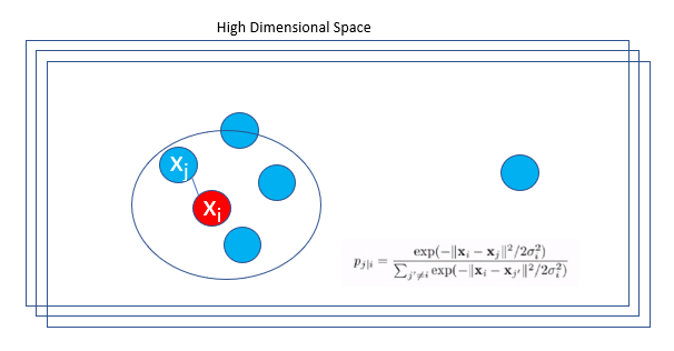
xᵢ would pick xⱼ as its neighbor based on the proportion of its probability density under a Gaussian centered at point xᵢ.

σᵢ is the variance of the Gaussian that is centered on datapoint xᵢ

The probability density of a pair of a point is proportional to its similarity. For nearby data points, p(j|i) will be relatively high, and for points widely separated, p(j|i) will be minuscule.

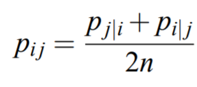
Symmetrize the conditional probabilities in high dimension space to get the final similarities in high dimensional space.

Conditional probabilities are symmetrized by averaging the two probabilities, as shown below.

Step 2: Map each point in high dimensional space to a low dimensional map based on the pairwise similarity of points in the high dimensional space.

The low dimensional map will be either a 2-dimension or a 3-dimension map

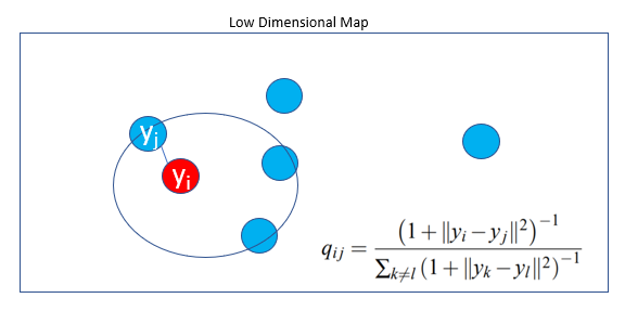
yᵢ and yⱼ are the low dimensional counterparts of the high-dimensional datapoints xᵢ and xⱼ.

We compute the conditional probability q(j|i)similar to P(j]i) centered under a Gaussian centered at point yᵢ and then symmetrize the probability.

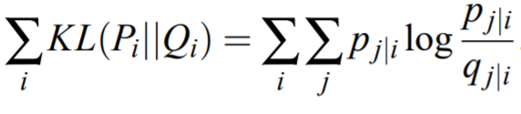
Step 3: Find a low-dimensional data representation that minimizes the mismatch between Pᵢⱼ and qᵢⱼ using gradient descent based on Kullback-Leibler divergence(KL Divergence)

t-SNE optimizes the points in lower dimensional space using gradient descent.

Why use KL divergence?

When we minimize the KL divergence, it makes qᵢⱼ physically identical to Pᵢⱼ, so the structure of the data in high dimensional space will be similar to the structure of the data in low dimensional space.

Based on the KL divergence equation,

• If Pᵢⱼ is large, then we need a large value for qᵢⱼ to represent local points with higher similarity.
• If Pᵢⱼ is small, then we need a smaller value for qᵢⱼ to represent local points that are far apart.

Step 4: Use Student-t distribution to compute the similarity between two points in the low-dimensional space.

t-SNE uses a heavy-tailed Student-t distribution with one degree of freedom to compute the similarity between two points in the low-dimensional space rather than a Gaussian distribution.

T- distribution creates the probability distribution of points in lower dimensions space, and this helps reduce the crowding issue.

How do I apply t-SNE on a dataset?

Before we write the code in python, let’s understand a few critical parameters for TSNE that we can use

n_components: Dimension of the embedded space, this is the lower dimension that we want the high dimension data to be converted to. The default value is 2 for 2-dimensional space.

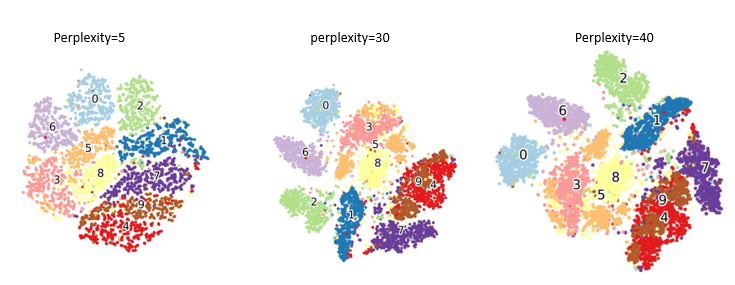
Perplexity: The perplexity is related to the number of nearest neighbors that are used in t-SNE algorithms. Larger datasets usually require a larger perplexity. Perplexity can have a value between 5 and 50. The default value is 30.

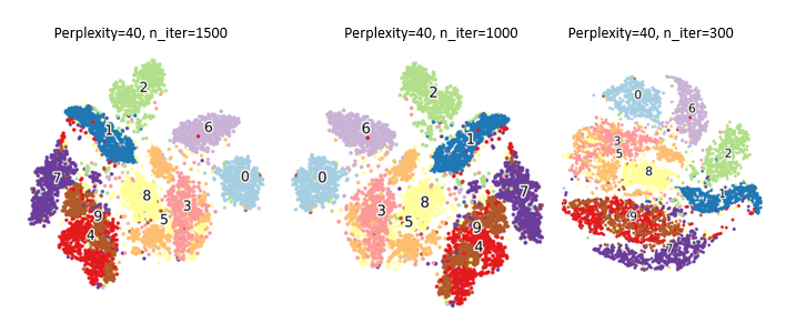
n_iter: Maximum number of iterations for optimization. Should be at least 250 and the default value is 1000

learning_rate: The learning rate for t-SNE is usually in the range [10.0, 1000.0] with the default value of 200.0.

Implementing PCA and t-SNE on MNIST dataset

We will apply PCA using sklearn.decomposition.PCA and implement t-SNE on using sklearn.manifold.TSNE on MNIST dataset.

Loading the MNIST data

Importing required libraries

import time
import numpy as np
import pandas as pd

Get the MNIST training and test data and check the shape of the train data

(X_train, y_train) , (X_test, y_test) = mnist.load_data()
X_train.shape

Create an array with a number of images and the pixel count in the image and copy the X_train data to X

X = np.zeros((X_train.shape[0], 784))
for i in range(X_train.shape[0]):
    X[i] = X_train[i].flatten()

Shuffle the dataset, take 10% of the MNIST train data and store that in a data frame.

X = pd.DataFrame(X)
Y = pd.DataFrame(y_train)
X = X.sample(frac=0.1, random_state=10).reset_index(drop=True)
Y = Y.sample(frac=0.1, random_state=10).reset_index(drop=True)
df = X

After the data is ready, we can apply PCA and t-SNE.

Applying PCA on MNIST dataset

PCA is applied using the PCA library from sklearn.decomposition.

from sklearn.decomposition import PCA
time_start = time.time()
pca = PCA(n_components=2)
pca_results = pca.fit_transform(df.values)

print ('PCA done! Time elapsed: {} seconds'.format(time.time()-time_start))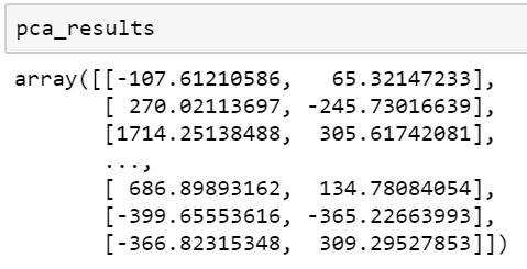

PCA generates two dimensions, principal component 1 and principal component 2. Add the two PCA components along with the label to a data frame.

pca_df = pd.DataFrame(data = pca_results
             , columns = ['pca_1', 'pca_2'])
pca_df['label'] = Y

The label is required only for visualization.

Plotting the PCA results

fig = plt.figure(figsize = (8,8))
ax = fig.add_subplot(1,1,1) 
ax.set_xlabel('Principal Component 1', fontsize = 15)
ax.set_ylabel('Principal Component 2', fontsize = 15)
ax.set_title('2 component PCA', fontsize = 20)
targets = [0,1,2,3,4,5,6,7,8,9]
colors=['yellow', 'black', 'cyan', 'green', 'blue', 'red', 'brown','crimson', 'gold', 'indigo']

for target, color in zip(targets,colors):
    indicesToKeep = pca_df['label'] == target
    ax.scatter(pca_df.loc[indicesToKeep, 'pca_1']
               , pca_df.loc[indicesToKeep, 'pca_2']
               , c = color
               , s = 50)

ax.legend(targets)
ax.grid()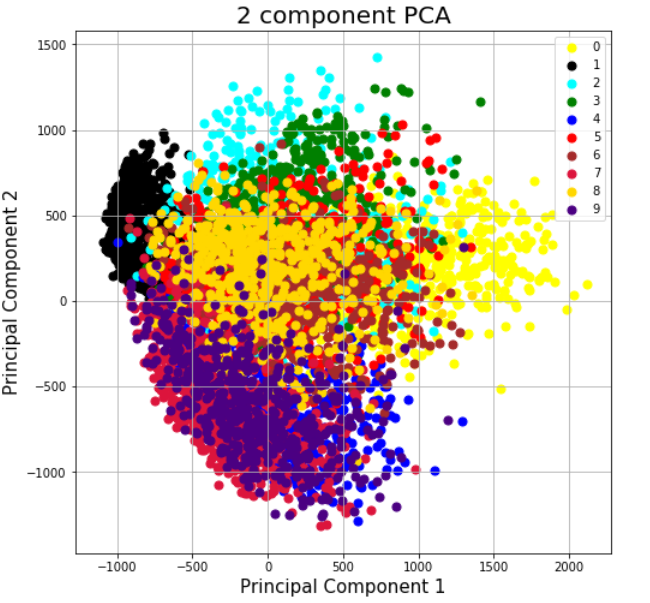

Applying t-SNE on MNIST dataset

Importing the required libraries for t-SNE and visualization

import time
from sklearn.manifold import TSNE
import matplotlib.pyplot as plt
from mpl_toolkits.mplot3d import Axes3D
import seaborn as sns
import matplotlib.patheffects as PathEffects
%matplotlib inline

Create an instance of TSNE first with the default parameters and then fit high dimensional image input data into an embedded space and return that transformed output using fit_transform.

The dimension of the image data should be of the shape (n_samples, n_features)

time_start = time.time()
tsne = TSNE(random=0)
tsne_results = tsne.fit_transform(df.values)

print ('t-SNE done! Time elapsed: {} seconds'.format(time.time()-time_start))

Adding the labels to the data frame, and this will be used only during plotting to label the clusters for visualization.

df['label'] = Y

Function to visualize the data

def plot_scatter(x, colors):
    # choose a color palette with seaborn.
    num_classes = len(np.unique(colors))
    palette = np.array(sns.color_palette("hls", num_classes))
    print(palette)
    
    # create a scatter plot.
    f = plt.figure(figsize=(8, 8))
    ax = plt.subplot(aspect='equal')
    sc = ax.scatter(x[:,0], x[:,1],  c=palette[colors.astype(np.int)], cmap=plt.cm.get_cmap('Paired'))
    plt.xlim(-25, 25)
    plt.ylim(-25, 25)
    ax.axis('off')
    ax.axis('tight')

# add the labels for each digit corresponding to the label
    txts = []

for i in range(num_classes):

# Position of each label at median of data points.

xtext, ytext = np.median(x[colors == i, :], axis=0)
        txt = ax.text(xtext, ytext, str(i), fontsize=24)
        txt.set_path_effects([
            PathEffects.Stroke(linewidth=5, foreground="w"),
            PathEffects.Normal()])
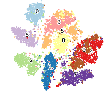
        txts.append(txt)

return f, ax, sc, txts

Visualize the -SNE results for MNIST dataset

plot_scatter( tsne_results, df['label'])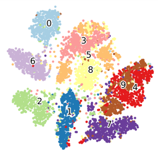

Try with different parameter values and observe the different plots

Visualization for different values of perplexity

Visualization for different values for n_iter

We can see that the clusters generated from t-SNE plots are much more defined than the ones using PCA.

• PCA is deterministic, whereas t-SNE is not deterministic and is randomized.
• t-SNE tries to map only local neighbors whereas PCA is just a diagonal rotation of our initial covariance matrix and the eigenvectors represent and preserve the global properties

Code is available here

Conclusion:

PCA and t-SNE are two common dimensionality reduction that uses different techniques to reduce high dimensional data into a lower-dimensional data that can be visualized.

References:

Visualizing Data using t-SNE by Laurens van der Maaten and Geoffrey Hinton.