
Principal Component Analysis (PCA)
In this article we will understand a technique called Principal Component Analysis(PCA)used to reduce the dimensionality when we have too many input features. We will understand what is PCA and how it works with a step by step example using Python

Prerequisites: Machine Learning
When we have a dataset with multiple input features we know the model will overfit. To reduce input feature space we can either drop or extract features
- Drop irrelevant, redundant features as they do not contribute to the accuracy of the predictive problem. When we drop such input variable we lose information stored in these variables.
- We can create a new independent variable from existing input variables. This way we do not lose the information in the variables. This is feature extraction
If we want to predict sales for a retail stores for a particular Item. Input features used for prediction are sales figures, retail changes of Item, inventory movement, store details, competitor’s retail, customer demography, and customer information like address, zip code etc.
We can drop certain variables like customer information. It does do not contribute to predicting sales for retail stores. When we drop these variables, we lose information available in those variables.
Principal Component Analysis -PCA help keeps the critical information in a dataset without dropping features. PCA does this by creating new independent variable from existing input variables.
What is Principal Component Analysis( PCA)?
When we have a large dataset of correlated input variables and we want to reduce the number of input variables to a smaller feature space. while doing this we still want to maintain the critical information. We can solve this by using Principal Component Analysis-PCA.
PCA reduce dimensionality of the data using feature extraction. It does this by using variables that help explain most variability of the data in the dataset
PCA removes redundant information by removing correlated features. PCA creates new independent variables that are independent from each other. This takes care of multicollinearity issue.
PCA is an unsupervised technique. It only looks at the input features and does not take into account the output or the target variable.
PCA helps with visualization of data by reducing the dimensionality of the dataset. If we have 9 input features and we visualize the data then the number of plot will be 9(9–1)/2=36. we have 36 different plots. As the number of input features increases the number of plots keeps increasing. It becomes difficult to look at all the plots and not all the plots will be informative. PCA reduce dimensionality by creating new variables. With reduced number of input features it is easy to visualize data.
PCA helps with faster and cost effective execution and less storage space. This is again possible with reduced input features.
Summarizing goal of PCA
Goal of PCA is to reduce the input feature dimension of the dataset from m to p where p
How does PCA work?
First step in principal component analysis is to standardize the input features. Different input features may be on different units. Standardizing input features puts them on the same unit scale.
After standardizing the data, we find the correlation or covariance between different variables.
Correlation shows if two variables have a relationship. If related do they have a positive or negative relationship.
we find the eigenvectors and eigenvalues by performing eigendecomposition using correlation matrix
What is eigenvalue and eigenvector and why do we need eigenvalue and eigenvector?
To reduce the dimensionality we need to select the input features with maximum variability. Eigenvalue determines the magnitude of the variability.
let’s understand briefly what is eigenvector and eigenvalue and how they help us understand variability in data
Eigenvector
Consider a matrix A to which we apply a linear transformation x such that
y =Ax
Here x is a vector that does not change direction along with linear transformation but the vector magnitude vary by λ such that
Ax= λx
λ is eigenvalue and x is eigenvector.
EigenValue
Eigenvalue determines the magnitude of the variability. Maximum eigenvalues signifies maximum variability. Eigenvector will lowest eigenvalues represent least information about the distribution of the data. we can drop eigenvectors with lowest eigenvalues.
Next we sorts eigenvalues in descending order. choose p eigenvectors with greatest eigenvalues. we choose a value for p less than the original input features m.
Finally we create a matrix Z from the selected p eigenvectors. Matrix Z forms our new reduced feature space.
We have finally transformed our original features to a reduced matrix Z and without losing information from the dataset.
Next question is how many principal components are we going to use for our new reduced feature space?
We use explained variance to determine how many principal components we should use
Explained variance is computed from eigenvalues. It is the measure of variance attributed to each principal component.
We can see from the plot below that the first two principal components are able to explain more than 90% of the information.
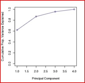
First principal component accounts for most variance present in the original data
Second principal component must be orthogonal to the first principal component. It captures the variance in the data that is not present in the first principal component
Summarizing steps for PCA
- Standardize the dataset
- Find the eigenvector and eigenvalues
- Sort the eigenvalues in descending order
- choose p eigenvectors will greatest eigenvalues where p< no. of features. p will be the feature subspace
- Create a matrix Z from the p selected eigenvectors
- we now have transformed our original features using matrix Z to have reduced p dimensional space
When do we use PCA?
- PCA should be used to reduce the input feature dimensionality when we are unable to identify variables that can be eliminated
- When we are comfortable with input features being less interpretable. PCA creates less interpretable new independent variables which are independent of each other.
- When we want all input variables to be independent of each other
A few things to consider when using PCA is that PCA is sensitive to outliers so we need to remove outliers.
Now we will take a simple array and run PCA step by step and also perform PCA using sklearn and compare the results.
we will first import the required libraries and create an array A of dimension 4 by 3. we have three input features in our array
import numpy as np
import pandas as pd
from numpy.linalg import eig
A =np.array([[100, 1, 1075],[125, 2,1900], [150, 1, 950], [91,1, 1650]])
print(A)output:[[ 100 1 1075]
[ 125 2 1900]
[ 150 1 950]
[ 91 1 1650]]we will first calculate the mean of each column mean_A
mean_A = np.mean(A.T, axis=1, dtype=np.int)
print(mean_A)output: array([ 116, 1, 1393])we now center the columns by subtracting from mean. Centering changes the value but not the scale
center_A= (A - mean_A)
print(center_A)output: array([[ -16, 0, -318],
[ 9, 1, 507],
[ 34, 0, -443],
[ -25, 0, 257]])Next we find the covariance of the centered array and then find the eigenvalue(value) and eigenvectors(vector) of the covariance. Eigenvalue with greatest number explains most variance in data.
covariance = np.cov(center_A.T)
value, vector = eig(covariance)
print(value.astype(int))output:[206898 630 0]we see that feature 1 and feature 2 have highest eigenvalue so we we need to use eigenvector for column 0 and 1 only
vector_with_highest_eigenvalue= vector[:,[0,1]]
PCA_calc = vector_with_highest_eigenvalue.T.dot(center_A.T)
print(PCA_calc.T)
output:[[ 317.63555359 -22.07788348]
[-506.73564035 18.70361328]
[ 443.56928479 25.52011189]
[-257.43119689 -20.07930745]]we now have transformed new features.
Now we use sklearn to compute the PCA and compare the PCA values with step by step approach values
import numpy as np
import pandas as pd
from sklearn.decomposition import PCA
pca= PCA(n_components=2)
pca.fit(A)
PCA_value= pca.transform(A)
print(PCA_value)output:[[-318.3760533 -22.59451704]
[ 505.99514063 18.18697972]
[-444.3097845 25.00347833]
[ 256.69069718 -20.59594101]]PCA values using sklearn is very close to the step by step calculation.
References:
An Introduction to Statistical Learning by Gareth James, Daniela Witten, Trevor Hastie, Robert Tibshirani


