SVMs for Non-Linearly Separable Data with Python

In our last few articles, we have talked about Support Vector Machines. We have considered them with hard and soft margins, and also how we can use the Kernel Trick when our data is not linearly separable. We have also seen how we can implement an SVM, with either hard or soft margin, in python when the data is linearly separable. However, in this article, we will only consider how to implement an SVM when our data is not linearly separable. . We will implement our models using Jupyter Notebook and various libraries.

Defining Our Data

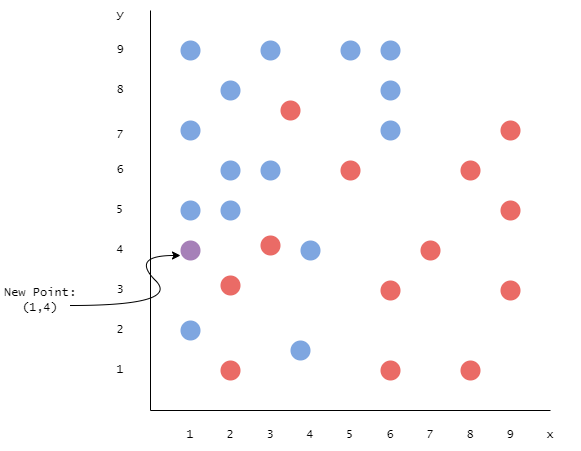
Before we can even dream about implementing our SVM, we first need to define some data. Imagine we have some data, which is distributed like so:

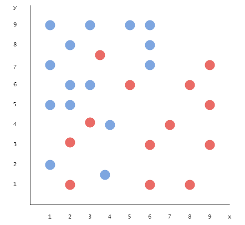
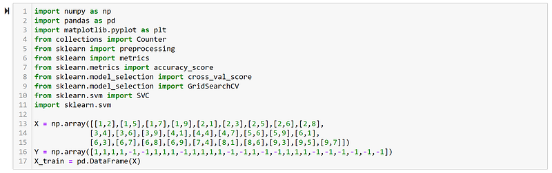
This data is clearly not linearly separable — so we will want to look at two ways to classify it anyway using a linear separating hyperplane. We will look at both how to do it using a linear SVM, but with a soft margin, or by using the Kernel Trick. However, we first need to define our data using code. We need to divide it into two arrays: X and Y. The X array consists of the data points coordinates and the Y array consists of their corresponding label. All of this would look like so:

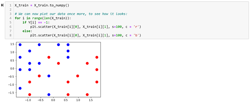
Let us now try to plot our data using matplotlib, and see if it resembles our draft of how the data should look:

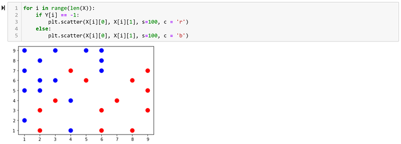
As we can see, it looks like it is supposed to look. We can now move on to the next part.

Normalizing the Data

We have now defined our data with code — however, that doesn’t mean that we are done with it yet! We still need to normalize it. Why is this important? It is because there sometimes is a big difference in scale between different input features. As an example, imagine that you have one feature which ranges between 0 and 10 while another ranges from 10.000 to 100.000. This means there is a great difference in the scale of our features, which can cause problems for some machine learning algorithms. Here, Support Vector Machines are one of these models. This is since Support Vector Machines assume that the data it uses is in a standard range, i.e., from either 0 to 1 or from -1 to 1. Therefore, it is important to normalize our data before using an SVM model on it.

Now, it is clear that our data probably doesn’t have a huge difference in scale between our two features (both range from 0–9), but we will normalize it anyway. We would want each of our two features to have a mean equal to 0 and unit variance. Let us see the code for it:

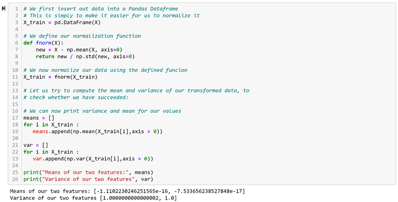
Here we can see that our means are practically zero, while our variances are also only negligibly different from 1. Let us see how this has affected how our data looks visually:

We can see that not much has changed, simply the scale of our features.

Building the Soft Margin SVM

We have finally come to the interesting part — building our machine learning model. We can start by building our soft margin SVM. Let us first try to remember how the optimization problem looks for the soft margin SVM:

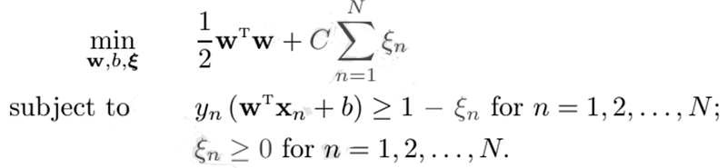
‘C’ is the penalty parameter for the Soft Margin SVM, or in other words, it determines how much it should punish our model for having points either misclassified or inside the margin. We can say that when C is large, then we care more about not violating the boundary than getting a large margin. This also means that we suddenly have to decide on which value of C is the optimal one for us. How can we do that? We can use a method called grid-search — we try to build models with different values of C, and then we cross-validate to find the best one. It would look like so in code:

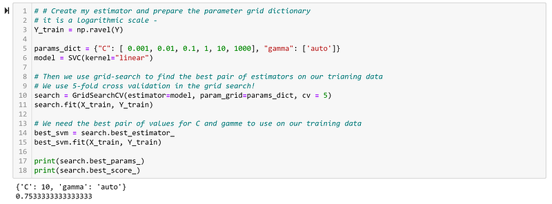
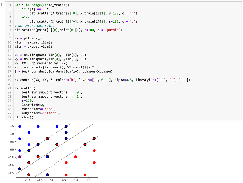
We can see that our best value of C is equal to ‘10’ and it gives an accuracy of 75.33%. It would also have been possible for us to have searched for the optimal value of ‘gamma’, but I chose to just use the automatic value. Let us now try to inspect the best model visually:

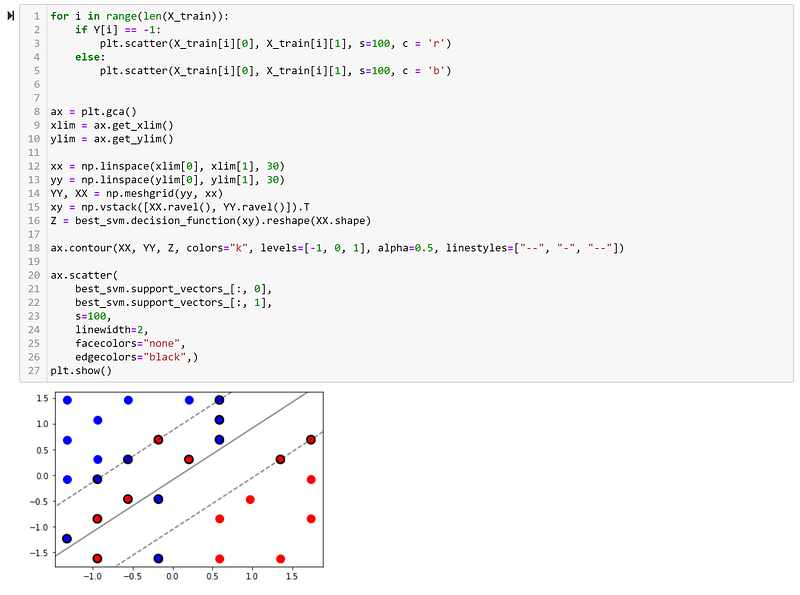
We can clearly see that we must accept some misclassification and points inside the margin.

So, what if we want to predict a new data point using our model? Imagine that we are given a new point, which is placed like so:

How would we use our model to predict its class? First of all, we would need to normalize it as well! However, we need to remember to normalize it using the training data. Let us see how it all looks in code:

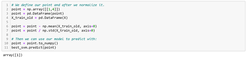
Hence, it would be classified as ‘1’ (blue). We can now see how it looks visually:

Building an SVM Using the Kernel Trick

We have now seen how we could still try to classify our data when it is not linearly separable by using the Soft Margin SVM. However, what if we instead use the Kernel Trick? We remember that we want to find a higher-dimensional space, where our data is linearly separable. For example, something like this:

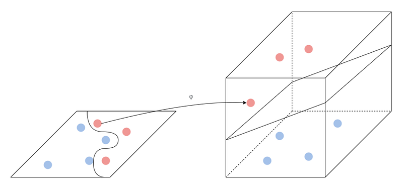
However, we also know that it can be computationally heavy if we really have to calculate every point in this new space. Therefore, we will simply use the Kernel trick. Our kernel function accepts inputs in the original (lower) dimensional space and returns the dot product in the higher dimensional space. Hence, we actually never need to transform all our data using the mapping function — we simply use the so-called Gram Matrix, which consists of these pairwise comparisons, in our calculations.

In this case, we imagine that we will use the ‘rbf’ kernel. We can again try to find the optimal value for ‘C’ using Grid Search. All of this is, luckily, very simple to implement using Python:

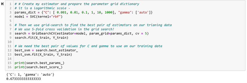
We can see that the optimal value for ‘C’ is equal to 1, while the model obtains an accuracy of 67.33%. Hence, it performs worse than our Soft Margin SVM.

We remember that ‘C’ is the penalty parameter for the Soft Margin SVM. It also means it must have an impact on how many data points lie within our margin — and maybe how many lay directly on the margin. Let us introduce two definitions:

• Free Support Vectors: Free support vectors lie on the margin.
• Bounded Support Vectors: All wrongly classified data points as well as the data points that are correctly classified but are inside the margin area are bounded support vectors.

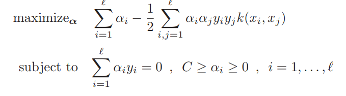
We would assume that when we have a high value of ‘C’, then we have fewer bounded support vectors than when we have a low value of ‘C’. Is there a way for us to check this? We can no longer do it visually, since our decision boundary has been found in a higher dimension space. That means that we need to do it mathematically. We will first need to look at the Dual Problem for our model, which looks like so:

Where we remember that α is our Lagrangian multiplier. Could we use it for something in our problem? As it turns out, yes. We have the following conditions that need to be satisfied when solving the optimization problem:

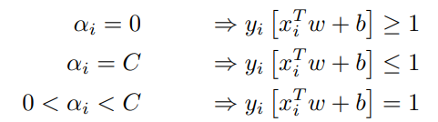
This means that we simply need to find the α-values of our model, and check their values. We can see that if α = C, then it is a bounded support vector and if 0 < α < C then it is a free support vector. Let us translate this into code:

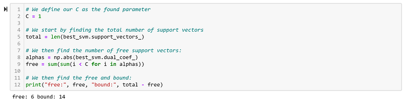
Now, we had an intuition that when we increased the value of C then we would have less points inside our margin. In other words, we would assume that we obtain less bounded support vectors. We can do this by simply creating classifiers with different values for C and then check the amount of bound and free support vectors as done above. Let us see how it would look with code:

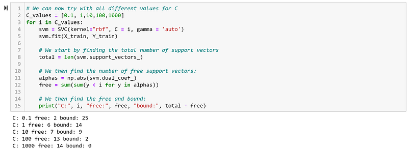
As we guessed, when we raise the value of C then we discourage having bound support vectors. We instead get free ones instead.

Conclusion

We have now seen how we can implement an SVM for non-linearly separable data. We could do this either through accepting a certain amount of misclassification, and therefore using a Soft Margin. We could also instead try to find a higher dimensional space, where we could see if our data would be linearly separable. We have also seen how we can check the amount of free and bounded support vectors in both cases.

References

• Igel, C. (2021). Support Vector Machines — Basic Concepts. In Machine Learning: Kernel-based Methods Lecture Notes (Version 0.4.3). Department of Computer Science University of Copenhagen.
• Seldin, Y. (2021). Vapnik-Chervonenkis (VC) Analysis. In Machine Learning Lecture Notes. Department of Computer Science University of Copenhagen.
• Ben-David, S. Shalev-Shwartz, S. Convex Learning Problems. Understanding Machine Learning: From Theory to Algorithms. Cambridge University Press.
• Abu Mostafa, Y. S. Magdon-Ismail, M. Lin, H.T. (2012). Support Vector Machines. In LEARNING FROM DATA — A Short Course. AMLbooks.com.
• Wilimitis, D. (2018). The Kernel Trick in Support Vector Classification. Medium.Com. https://towardsdatascience.com/the-kernel-trick-c98cdbcaeb3f
• Bosnalı, C. (2018). Support_Vector_Machine_from_Scratch. GitHub.Com. https://najamogeltoft.medium.com/an-introduction-to-continuity-and-the-intermediate-value-theorem-700ec10f6ba1