
Understanding The Kernel Trick In Machine Learning — Part 2
In the former article, Part 1, we didn’t even get to hear anything about these so-called kernels and what trick they can perform. All we heard about was linear classification and how we could calculate the decision boundary. Well, despair not — all this knowledge will be used and/or extended upon in this article and in coming articles. However, in this article, we will finally talk about kernels and the helpful tricks they can perform for us.
Defining Hyperplanes
Before you get too excited, we will first start by talking about hyperplanes. This is since we will replace our term ‘decision boundary’ with ‘separating hyperplane’. Why? Because in this article we will need to start considering the dimension our data exists in — and because in later articles we will start talking about Support Vector Machines, where the decision boundaries are referred to as separating hyperplanes.
So, let us revisit our example from the former article. Here, we found our decision boundary to be equal to:

This meant that our decision boundary was simply a straight line. However, what will happen when our data gets more dimensions, i.e., we have to consider more and more inputs? It will mean that our boundary is no longer a simple line — it instead becomes a plane (in the case of 3-dimensional data) or a hyperplane (in the case of more than 3-dimensional data). As it turns out, our separating (hyper)plane is always in one dimension less than our data.
For the sake of clarity, let us take an illustrative example. Imagine that we now have 3 inputs for each data piece. This also means that we need 3 weights, and we have found they and the bias are equal to:
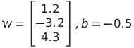
We can then calculate the boundary to be equal to:
This is the equation for a plane, which by definition is a 2-dimensional surface. Hence, our 3-dimensional data can be classified by using a 2-dimensional surface, in other words, the plane separates our data into two classes. If we had gone up in dimensions, i.e. considered more inputs, then our plane would have become a hyperplane. It has now, hopefully, become clear why we will now refer to the decision boundary as the separating hyperplane. For sake of ease, the line and the regular 2-dimensional plane are also included in this term.
The Motivation For Kernels
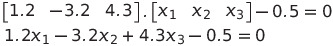
Now that we have cleared this, let us then understand the motivation behind kernels. Do you remember those annoying cases in the former article, where it was impossible for us to find a straight line, which could separate the two classes completely?
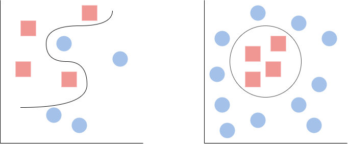
How could we possibly solve this problem? Of course, we could simply use something more complex than a linear classifier — as shown above. However, what if we really do want to use a linear classifier? Imagine if we could instead find a higher dimensional space in which these points were linearly separable. Let us see an example:
Here we can see that we have mapped our points from a 2-dimensional space into a 3-dimensional space. It has then made it possible for us to find a separating hyperplane, which can linearly separate the points. This is done by feature mapping, i.e., mapping our features from one space to another.
Introducing Feature Mapping
So, we have now clearly seen that it is possible for us to transform our data from a lower dimension into a higher, by using a so-called feature map. We will denote our feature map by the symbol ‘ϕ’. Let us first try to define it formally, then we can afterward understand it more intuitively.
We will first denote our input space as X, which is simply the space our inputs ‘live’ in. Then we will denote the feature space as F. Then we can say that our feature map is simply written as:

What does this mean? It means that our feature map is nothing more or less than a function. It is a function that maps our data in the input space to the feature space. Let us try to take an illustrative example.
Imagine that we have some data, which exists in a 2-dimensional space. We then want to define a feature map, ϕ, which transforms it into 3-dimensional data. In other words, we have:

We can then define the feature map exactly to be equal to:
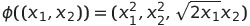
We have then created a completely new set of coordinates. Now, let us try to see the impact of some data. Imagine that we have the following data:
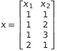
Then we can see how our feature map transforms it:
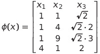
We have now seen how a feature map is nothing more than a function, which simply takes our original data and maps into a new space. Here, of course, we simply used our own home knitted feature map — there are an infinite amount of different ones! This also means that (1,1) in our original space corresponds to (1,1, √2) in the new space, and vice versa.
Your question might then be: “Ok, so how are feature mapping and kernels connected to each other? Because if I remember correctly, it is called the kernel trick and not the feature mapping trick”. Well, let us first consider the viability of feature mapping.
Imagine that you have a dataset with hundreds of thousands, maybe even millions, of samples. This dataset is not linearly separable, hence you decide to use feature mapping to transform your data into a higher dimension. Now, what could be the problem with this? For one, this is a very expensive computation to make — both timewise and memory-wise! And the problem only gets worse the more data you amass, or the higher dimension you want to map to. So, clearly, the solution is not perfect. Is there possibly some way that we can keep the good part of feature mapping, i.e. finding a higher dimension space where the data is linearly separable while scrapping the bad parts?
Pairwise Comparison Functions
Now, imagine this: Instead of actually calculating the new coordinates, we instead find a function that returns the inner product between the images of two inputs in some feature space. This is without even having to know the given feature space, or calculating a single coordinate. We will get to that later. But, in other words, we are looking for a pairwise comparison function, since dot product can be seen as how similar two vectors actually are. This is where kernels come into the picture.
Let us start by defining a kernel. A kernel is a comparison function, which takes a set of data points and uses a given comparison function and compares all the data points pairwise. These pairwise comparisons are presented in a matrix, specifically a Gram Matrix. Now, let us try to make it a tinge more formal. We can first define our comparison function, K:

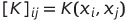
This simply means that we always consider the same space, our input space, X, and we spit out a real number. So, let us imagine that we have a data set, S, which exists in our input space, X. In this dataset, S, we have n points. We then need to compare each point pointwise to every point in the dataset, including itself. Since we have n points in our dataset, this results in a matrix with dimensions equal to n x n. The matrix can mathematically be defined as:
Let us take an illustrative example to understand the idea better. Imagine that we have a dataset, D, which consists of 3 data points:

We then need to compare each point pointwise with each point in the dataset, including itself. This results in a matrix, which looks like so:
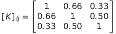
For example, when we compare ‘abc’ itself then it is equal to 1 since they are completely similar. However, when we compare ‘abc’ to ‘and’ then it is only 0.33 similar.
Positive Definite Kernels
Now, we will limit ourselves to a certain type of pairwise comparison functions. These functions are called positive definite kernels. Let us first look at the formal definition of positive definite kernels:
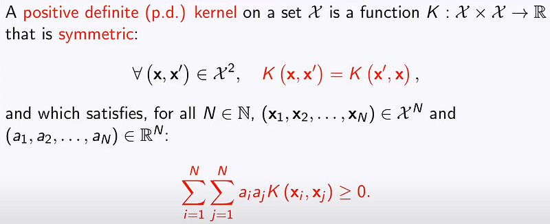
So, we remember it is still a comparison function, which operates on the input space, X. However, it has to fulfill two demands:
- Symmetry: It has to be symmetric, such that K(x, x’) and K(x’,x) are equal to each other. If we remember our example, it simply means that we need to get the same result when we compare ‘abc’ to ‘and’ and when we compare ‘and’ to ‘abc’.
- Positive Semi-definite: Remember the matrix we could construct, the Gram Matrix, should be positive semi-definite. This simply means that the eigenvalues of the matrix should be non-negative.
We will extend some more upon these positive definite kernels. Let us first look at a mathematical lemma:
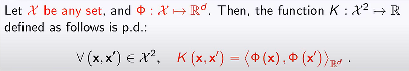
What does this say? Imagine that we have some data which exists in a space, X. We are also given a feature map, ϕ, which takes our data to an euclidian space (R^d). We then know that we need to find the inner product, i.e. the pairwise comparisons, in our feature space. This is equal to writing:
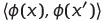
Then the lemma states that this is equal to a positive definite kernel. This might not seem super exciting, but this next information is. The opposite holds true as well. If we have a positive definite kernel, then there also exist an euclidian space and a mapping, ϕ, such that it is equal to the inner product of our mapped data in the feature space. What we have now shown is that our positive definite kernel can simply be written as the inner dot product between our feature mappings of two given points.
From Feature Mapping To Kernels
So, what exactly have we learned? What we have learned is the kernel trick. The “trick” in this is that kernel method represents the data only through a set of pairwise similarity comparisons between the original data points, x, instead of actually applying the transformations ϕ(x).
This data is represented in the so-called Gram Matrix of dimensions n x n. Here the entries (i, j) are defined by the kernel function:

Our kernel function accepts inputs in the original (lower) dimensional space and returns the dot product in the higher dimensional space. Hence, we actually never need to transform all our data using the mapping function — we simply use the Gram Matrix, which consists of these pairwise comparisons, in our calculations. All of this is allowed, since we have shown how positive definite kernels is equal to the inner product of our mapped data in the feature space.
Creating More Positive Definite Kernels
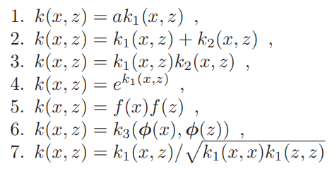
We have clearly seen that our kernels need to be positive definite to be able to used in this manner. We also saw that there are two conditions for a kernel to be positive definite. However, we might sometimes be lazy to check whether our kernel actually fulfills these demands — and therefore can be used. Hence, it is useful to know how to derive new positive definite kernels from other positive definite kernels. Imagine that we have the following kernels which we have proved to be valid:

Then the following functions are positive definite kernels:
Conclusion
We have now gotten a small introduction to Kernel Methods and the so-called Kernel Trick. We have seen how it can save us many computations, when we want to project our data into a higher dimension while looking for a separating hyperplane. In the next few articles, we will look at the theory behind Support Vector Machines. This is since we can afterwards show how SVM’s use kernel methods.
References
- Igel, C. (2021). Support Vector Machines — Basic Concepts. In Machine Learning: Kernel-based Methods Lecture Notes(Version 0.4.3). Department of Computer Science University of Copenhagen.
- Abu Mostafa, Y. S. Magdon-Ismail, M. Lin, H.T. (2012). Support Vector Machines. In LEARNING FROM DATA — A Short Course. AMLbooks.com.
- Wilimitis, D. (2018). The Kernel Trick in Support Vector Classification. Medium.Com. https://najamogeltoft.medium.com/an-introduction-to-continuity-and-the-intermediate-value-theorem-700ec10f6ba1
- Mairal, J. (2021). Lecture 1 on kernel methods: Positive definite kernels. Youtube.Com.https://www.youtube.com/watch?v=IzGS8uKc5E4&t=1865s&ab_channel=JulienMairal


