StyleGAN Image Generation: A Comprehensive Guide for Beginners

From Basics to Implementation: Mastering StyleGAN with PyTorch

AI image generation has been a widely discussed topic in recent times, both in the realm of art and machine learning. Recent AI tools like Dall-E, Midjourney, and others are constructed based on a generative model called the ‘Diffusion model’.

However, generative models in the field of image generation are not limited to just the diffusion model; there are other remarkable approaches such as VAE, GAN, Flow-based models, and more.

In my previous article, I provided a brief overview of the mathematical principles behind the diffusion model and how to implement it using PyTorch. This time, let’s switch gears and explore another popular generative model: Generative Adversarial Networks (GANs).

In this article, I will provide a detailed explanation of the architecture and training process of the GAN model. We will be building our image generation model based on Nvidia’s StyleGAN, which was introduced in 2019.

As this article is for beginners, we won’t delve into complicated mathematics. The goal is for everyone to enjoy training their own generative model after reading this. 👏 👏

Table of Contents

· Table of Contents · What is Image Generation? · Data Distribution · Latent Space & AutoEncoder ∘ AutoEncoder · Generative Adversarial Network ∘ Loss Function ∘ Training Step · The problem with classic GAN · Style Generative Adversarial Network · Why Mapping Network? · Synthesis Network · Conclusion · Reference

What is Image Generation?

Before we delve into the main topic, let’s first discuss a question: What is image generation? Or, in other words, what exactly is an image, and how can it be generated?

An image in a computer is stored in the form of a three-dimensional array. For example, a 64x64 RGB image is represented as a three-dimensional array with shape [64, 64, 3]. It means that this image is composed of 64x64x3 = 12,288 numbers in total.

So, to create an image, we only need to sample 12,288 numbers randomly following a specific probability distribution. But now comes the question, how do we obtain that ‘specific probability distribution’?

Data Distribution

In supervised learning, the data we use is a sample from the real data distribution, or you can say it’s a sample from the population.

Each sample is often characterised by multiple values, which are referred to as “features”. When we assume that each feature is independent of the others, we can construct a high-dimensional distribution space with each feature serving as an axis.

For example, consider a dataset containing information about individuals in a city. Each individual includes:

1. Age
2. Income
3. Education Level

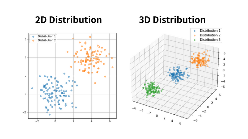
Based on the provided information, if we select only two features (age and income), we can establish a 2D distribution space (left image) where each individual corresponds to a single ‘point’ within this space.

As we incorporate more features, we can extend this concept to higher-dimensional spaces, where each sample is scattered throughout this space as a “point.”

Furthermore, when these sample points in the high-dimensional space are close enough to each other, they form what we call a “Distribution”.

Since data with similar “features” tend to belong to the same distribution, when addressing a classification problem, our goal is to classify the data into this distinct distribution rather than classifying the data points individually.

By understanding the concept of data distribution, we can interpret an image as a data point located in 12,288-dimensional space

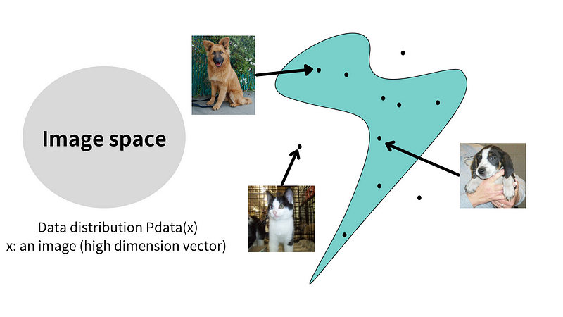
In addition, if we gather a large collection of image data, for example, 64x64 dog photos, and project them into this 12,288-dimensional space, all of the dog images will belong to the same distribution, as these photos share the same attribute, which is being ‘dog’ photos

So, to generate a new image, we only need to know what the image distribution exactly is, or more specifically, we only need to obtain the probability density function (PDF) of the image distribution.

Latent Space & AutoEncoder

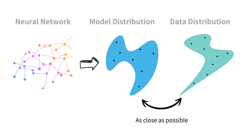
In order to simulate the probability distribution of real-world data, often denoted as Pdata(x). A common approach is to use a neural network to approximate a model’s distribution Pmodel(x). The goal is to minimise the distance between Pdata and Pmodel, ensuring they are as close as possible.

To build our model, we can utilise the architecture of an auto-encoder, an Encoder-Decoder architecture.

AutoEncoder

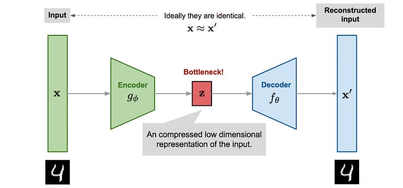
An auto-encoder is a neural network architecture used in unsupervised learning and data compression. It consists of an encoder that compresses input data into a lower-dimensional representation and a decoder that reconstructs the original data from this representation.

This “lower-dimensional representation” is commonly known as a“latent vector”, while the space in which they are located is called the“latent space”.

Given that the latent vector contains all the essential information required for the decoder to reconstruct an image, can we generate a new image by modifying the latent vector ❓❓

Now, let's try to implement it~~

This is a simple model that is mainly composed of Linear layers, we use the handwritten digits dataset MNIST to train our model.

The encoder will map the input image into a 2-dimensional latent space, while the decoder will recover the image from the latent. Mean Square Error was used to compare the difference between real and fake images.

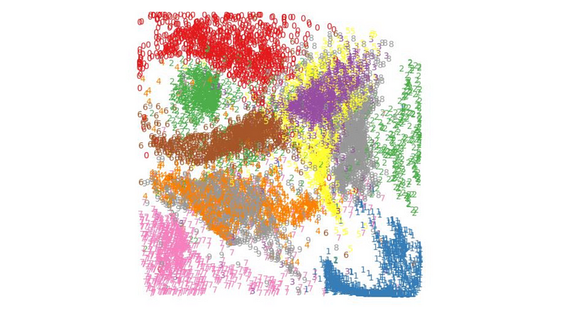
Now let's call the encoder and see how the image looks like within the latent space ~~

We can observe that the encoder encodes different numbers into different locations; for example, the number one appears at the right bottom, while the number seven is located at the left bottom, and so on.

Finally, let’s randomly sample some latent vector, and generate image through decoder 😙😙

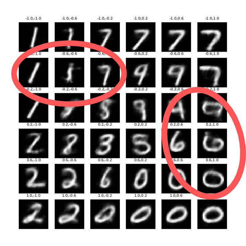
The digits shown above are generated by the decoder, where the two values represent the two inputs of the latent vector. We can see that the decoder can generate numbers quite well for most latent vectors.

However, when our latent vector falls between two distributions (the red circle part), the decoder will start to blend two different numbers.

For example, in the top left corner, the decoder tries to generate a number that falls between 1 and 7, which results in the 1 in the middle appearing somewhat distorted. 😢

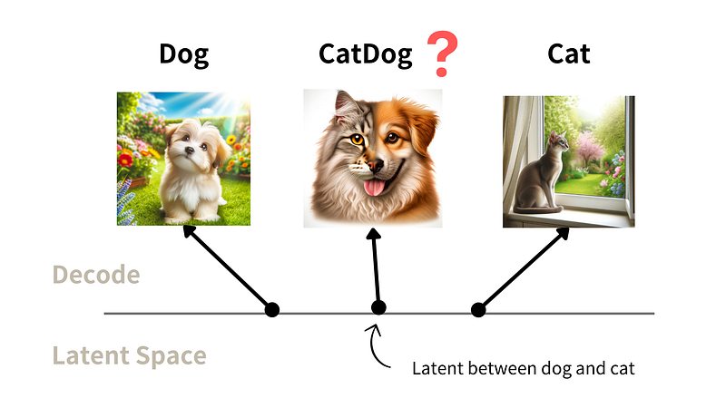
To solve this problem, let me introduce a more advanced method: Generative Adversarial Network !!! 👏 👏

Actually, there is an improved version of the auto-encoder called Variational Auto-encoder that can address this issue. If you’re interested, you can refer to this paper

Generative Adversarial Network

The concept of generative adversarial networks (GANs) was first introduced in the paper “Generative Adversarial Networks” by Goodfellow et al. in 2014.

An Adversarial Net consists of two main components: the generator, which is responsible for creating images, and the discriminator, which checks these images to see if they are real or not.

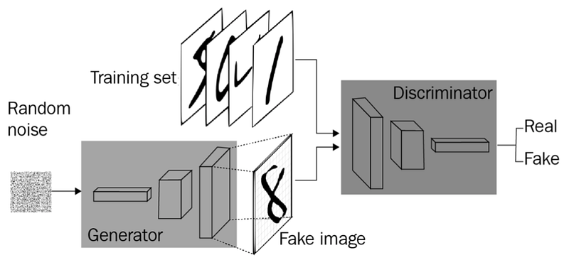
• Generator: tries to fool the discriminator by generating real-looking images
• Discriminator: tries to distinguish between real and fake images

The generator of GAN can be seen as the decoder of an auto-encoder. However, the key difference is that GAN incorporates a discriminator component to evaluate the quality of images generated from the generator, preventing the generation of implausible or unrealistic images.

Loss Function

• G: generator
• D: discriminator (output a value between 0 ~ 1, fake:0, real:1)
• X: an image (a high dimension vector)
• Z: latent vector (random sample from Gaussian distribution）

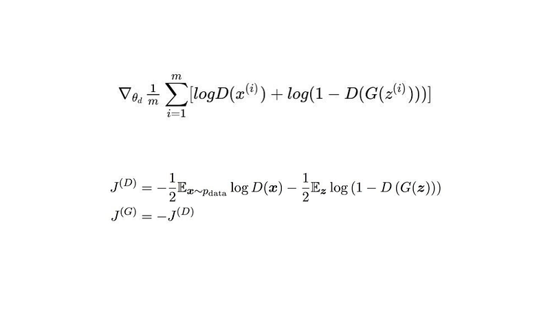
The GAN loss function sets different goals for the generator and the discriminator, creating competition between them.

The discriminator tries to get better at telling real images (maximising logD(x)) from fake ones made by the generator (minimising log(1-D(G(z)))), while the generator’s aim is to trick the discriminator, doing the opposite of what the discriminator does.

This adversarial setup (JG = -JD) is why it’s called “Adversarial Network”: the generator and the discriminator have opposite objectives and are in a constant battle against each other. 🤜🤛

The code above is the loss of GANs. You might wonder if the loss for the generator should be “1 — D(G(z))”. In fact, in the original GAN framework, the loss was indeed defined as “1 — D(G(z))”.

However, this loss function can lead to a problem known as generator saturation, where the gradients become too small to effectively train the generator.

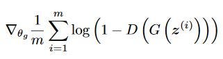
To address this issue, some modifications have been made to the original loss function. Instead of minimising the probability that a generated image is classified as fake, the generator is encouraged to maximise the probability of its images being classified as real. This method is known as the Non-Saturating GAN Loss [-log(D(G(z)))].

Training Step

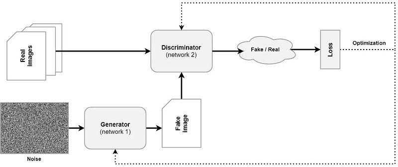
1. Generator generates images from random noise (z)
2. Input real or fake images to the discriminator, and then the discriminator will output a scaler indicating the likelihood of the image being real.
3. Calculate the loss based on the output from the discriminator and then update the model’s weights.
4. Repeat the process until the model converges.

Now, it’s time for some coding ‼️

In this implementation, we will use the CelebA-HQ dataset to train the model, resizing the images to a 64x64 resolution and normalising their values to range between -1 and 1.

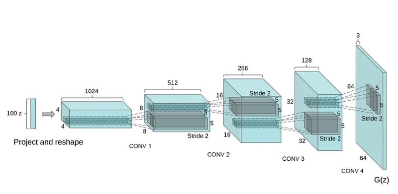
The generator and discriminator both employ a deep convolutional architecture. The discriminator uses stacked CNN layers to identify features and classify images, while the generator does the opposite, up-sampling the latent vector to reconstruct the image.

The training loop is simple: we compute the loss and update the model weights for both the generator and discriminator. A notable modification is the addition of a gradient penalty to the discriminator, while the generator is updated every 5 steps. This approach is derived from WGAN-GP, which aims to enhance training stability. For more details, I recommend reading the official paper.

The problem with classic GAN

Although classic GAN has provided remarkable performance in many computer vision tasks, there are some issues that need to be addressed:

1. The training process is unstable

2. It’s difficult to control the style of the generated images

For the first issue, it is caused by the process of training two models simultaneously; if one model is too strong or too weak, it can lead to training instability. This problem can be addressed by applying gradient penalties to the discriminator. (WGAN-GP)

Regarding the second issue, it is caused by the entanglement of our latent space (z). To address this problem, we can use the model I will introduce next, StyleGAN.

Style Generative Adversarial Network

The Style Generative Adversarial Network, or StyleGAN for short, is an extension of the GAN architecture first proposed by Karras et al. (2018). Which introduces two new structures: Mapping network and Synthesis network.

• Mapping Network: Utilise multiple fully connected (FC) layers to map the latent vector z to the space that fits the network better.
• Synthesis Network: Concate the latent vectors across all layers to control image style, deviating from traditional GANs, which start with a fixed constant.

Why Mapping Network?

In the previous section, I mentioned that controlling style through latent variables becomes challenging if the latent space is “entangled”. Therefore, it’s necessary to “disentangle” the latent space. Now, let me explain what is the term entanglement ~~

When we want to control a specific feature of an image, such as the hair length of a male, we often assume that this can be achieved by adjusting a single component of the latent vector.

However, there is no guarantee that each latent component controls only a single feature due to “entanglement”. For instance, if a component affects both hair length and gender, modifying it could lead to an unexpected result, such as a female with long hair. To address this issue, it’s necessary to ensure that each component exclusively manages a single feature, a process known as disentangling.

In StyleGAN, we can easily disentangle the latent space by introducing a mapping network composed mainly of fully connected (FC) layers ! 😄😄

Synthesis Network

StyleGAN introduces a unique feature in its synthesis network. Unlike traditional GANs that use latent vectors directly to generate images, StyleGAN uses these vectors to adjust the style of the image.

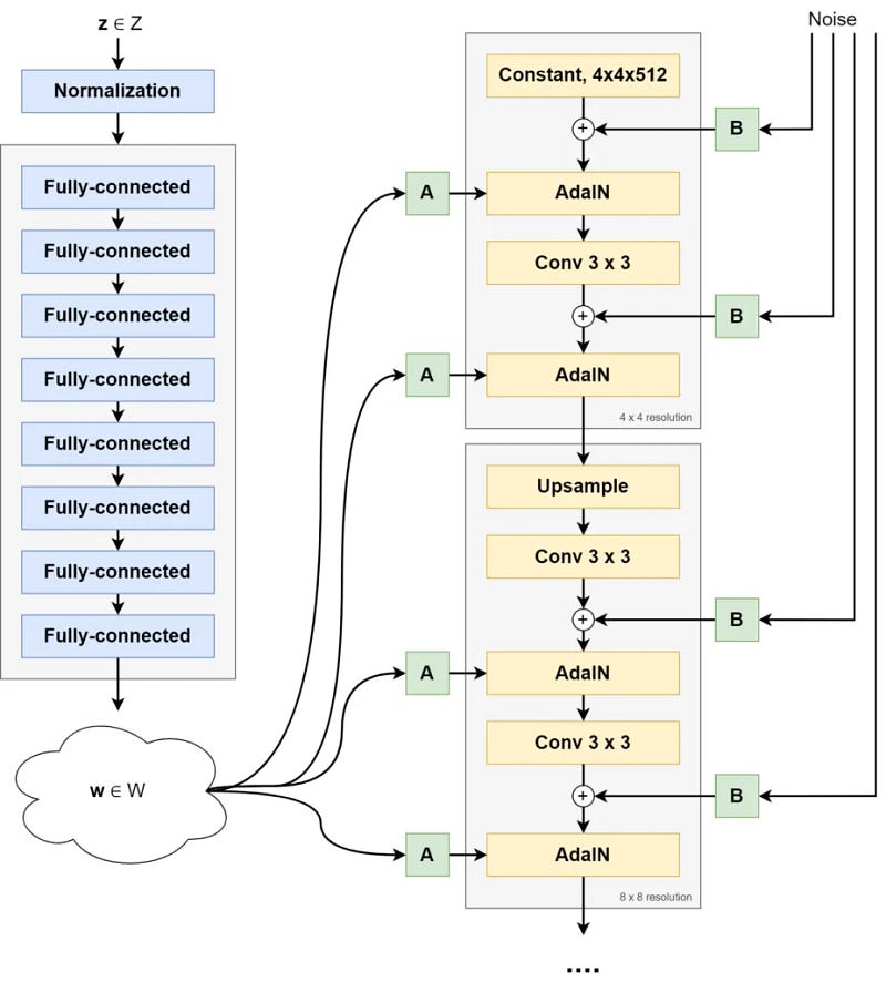
The latent vector w in StyleGAN is applied across all layers. This means that w is mainly used for style changes at each layer. The starting point of the network is a fixed constant, which is different from classic GANs.

Moreover, since image generation in StyleGAN begins with a fixed constant, to ensure diversity in the outcomes, StyleGAN adds noise to every style block, introducing randomness into the model.

Finally, here is the code for G_block and Generator !! ✋ ✋

That’s all about the StyleGAN ❗️ The Discriminator and the training loop are mostly the same as in a classic GAN. If you are interested in the full implementation, feel free to refer to my GitHub: click on me

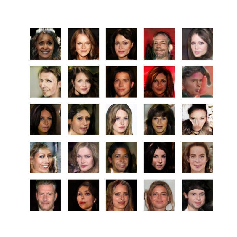
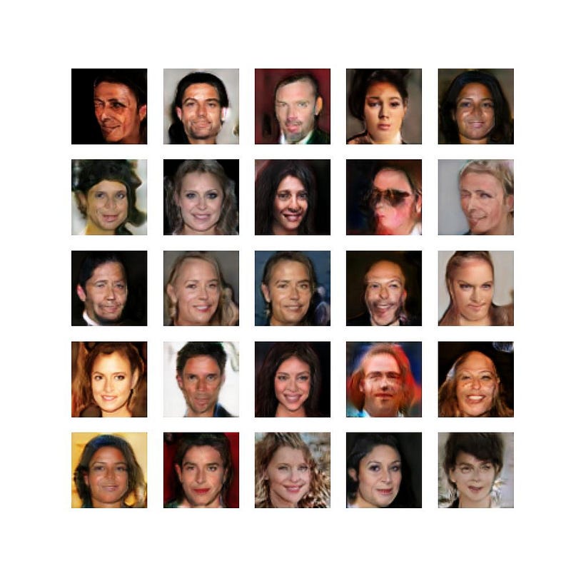
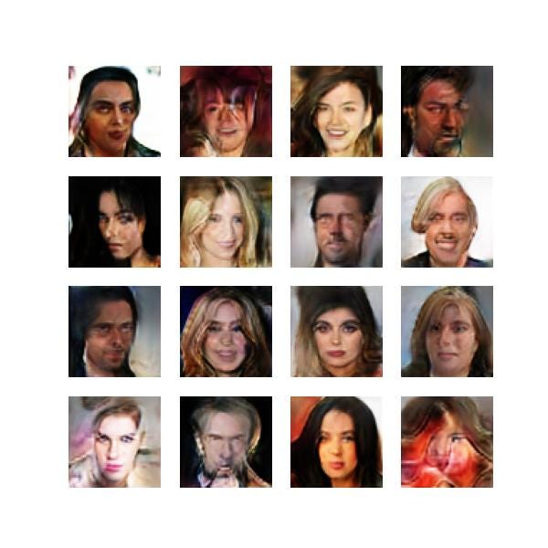
Above is the result after 6 hours of training. We could see that although the model has not converged very well, leading to some distorted images. However, we are still able to generate high-quality facial images.

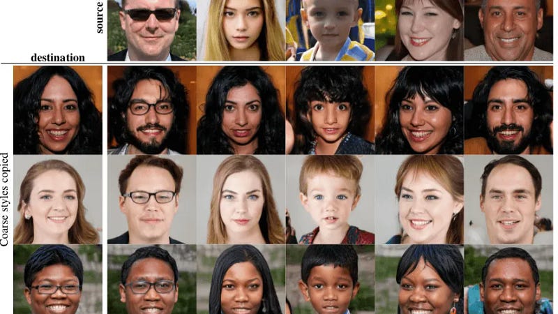
Furthermore, by mixing inputs from different style layers, we can control the images’ style, which is why this model is referred to as a ‘Style’ GAN.

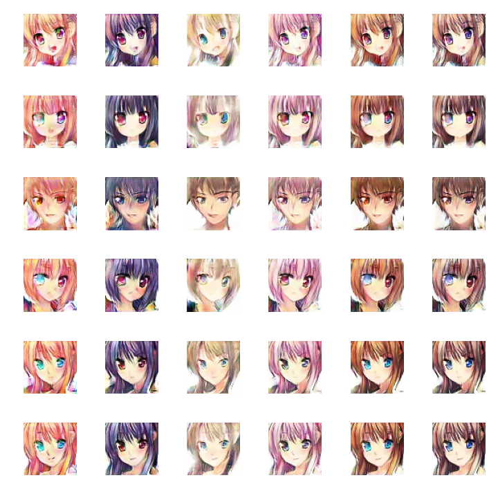
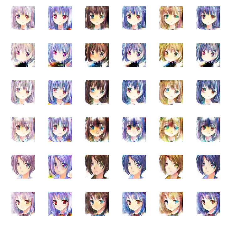
By modifying the style of the last style block (5 in total), we can control the hair colour of the character. ~~ 😄

Conclusion

In this article, I cover the whole process of image generation, beginning with the concept of data distribution and then using auto-encoders for image creation. Lastly, I talk about a very popular and effective model in computer vision, known as the Generative Adversarial Network, while also introducing its variation, StyleGAN.

If you’re interested in learning more about StyleGAN, I recommend reading the paper: StyleGAN2. StyleGAN2 is an improved version of StyleGAN, primarily aimed at fixing the problem of blob-shaped artifacts. The main modifications include adjustments to AdaIN and the use of lazy regularisation, along with other updates.

~~~~~~~~~~~~~~

Finally, I hope you enjoyed this article. I will write more articles related to AI, including explanations of their underlying principles and how to implement them.

If that sounds interesting to you, feel free to follow me. 👏 😁

My Medium: link

My LinkedIn: link

Reference

1. Kingma, D. P., & Welling, M. (2013). Auto-encoding variational bayes. arXiv preprint arXiv:1312.6114.
2. Goodfellow, I., Pouget-Abadie, J., Mirza, M., Xu, B., Warde-Farley, D., Ozair, S., … & Bengio, Y. (2014). Generative adversarial nets. Advances in neural information processing systems, 27.
3. Karras, T., Laine, S., & Aila, T. (2019). A style-based generator architecture for generative adversarial networks. In Proceedings of the IEEE/CVF conference on computer vision and pattern recognition (pp. 4401–4410).
4. Karras, T., Laine, S., Aittala, M., Hellsten, J., Lehtinen, J., & Aila, T. (2020). Analyzing and improving the image quality of stylegan. In Proceedings of the IEEE/CVF conference on computer vision and pattern recognition (pp. 8110–8119).