
Understanding the Diffusion Model and the theory behind it
Tensorflow implementation with explanation
AI image generation is a technology that has been hotly discussed in the art and Deep Learning (DL) field. You must have heard of the AI Art Generator such as Dall-E 2 or NovelAI, a DL model that generates realistic-looking images from a given text sequence.
To explore this technology deeper, we need to introduce a new class in the generative model called ‘diffusion’, first proposed by Sohl-Dickstein et al. (2015), which aimed to generate images from noise using a backward denoising process.
So far, several generative models exist, including GAN, VAE and Flow-based models. Most of them could generate a high-quality image, such as StyleGAN-XL, the current State-of-the-Art image generation model. However, each has some limitations of its own.
GAN models are known for potentially unstable training and less diversity in generation due to their adversarial training nature. VAE relies on a surrogate loss. Flow models have to use specialized architectures to construct reversible transforms (Lilian Weng, 2021)
The diffusion model has provided a slow and iterative process when noise is converted into an image; this makes the diffusion model more scalable than the GAN model. Besides, since the target of the diffusion model is to predict the input noise, which is supervised learning, we could expect the training of the diffusion model will be much more stable than GAN (unsupervised learning).
The implementation in this article will be based on Denoising Diffusion Probabilistic Models (Ho et al., 2021) (DDPM) and Denoising Diffusion Implicit Models (Song et al., 2021) (DDIM).
Table of Content
· What are Diffusion Models? · Forward Noising ∘ Property 1: Reparameterization trick ∘ Property 2: Xt at any timestep can be represented by X0 and β ∘ Mathematical proof of Property 2 · Backward Denoising ∘ DDPM ∘ Mathematic behind the reverse process · Model Architecture and Training ∘ U-net blocks ∘ U-net model ∘ Training · Result · Reference
What are Diffusion Models?
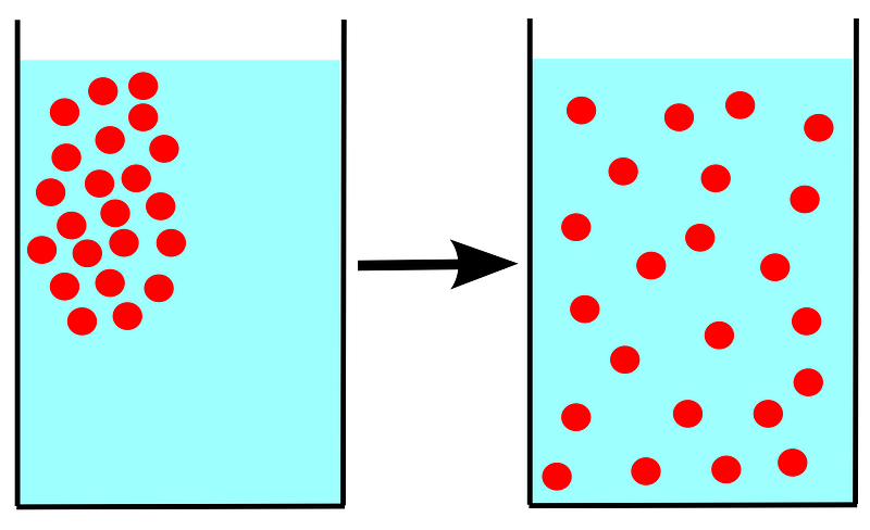
The word diffusion was defined as the movement of any substance from a higher concentration region to a lower concentration.
Inspired by this concept, the diffusion model defined Markov chain to slowly add random noise to the image. The Markov chain could be seen as a diffusion, and the process of adding noise is the movement. Thus, our target is to find the noise (movement) added to the image and reverse this process.
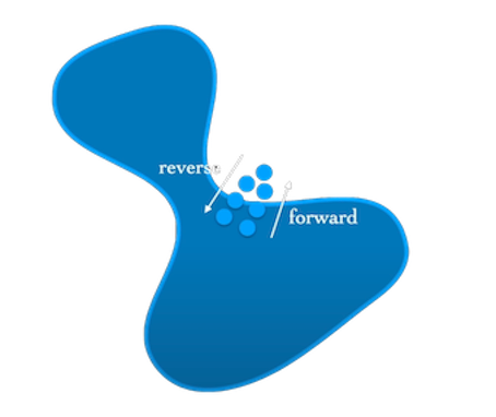
The diffusion model is mainly composed of two processes Forward Noising and Backward Denoising; this could be regarded as continuously adding noise into the image than reversing this process. 😈 😈
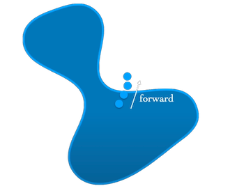
Forward Noising
In the DDPM paper, the author defines the forward process as:
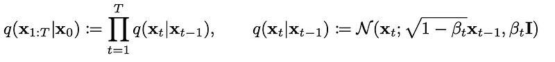
The above is a Markov chain in which every timestep t only depends on the previous step t-1. We use variance schedule β to control the mean and variance, Where β₀ < β₁< … < βt.
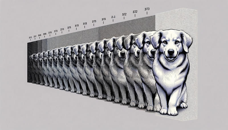
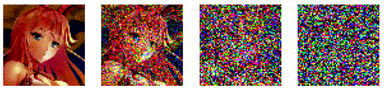
We will start from x0 (sampling from the real data distribution q(x) ) and then resign the mean and variance of x0 to generate x1. Finally, to the final state xT, which is a Gaussian noise. This process could be seen as pushing the image out iteratively until it leaves real data distribution and becomes noise.
Before we start coding, let me first introduce two important properties in the diffusion model.
Property 1: Reparameterization trick
In the diffusion model, we will have a lot of values that need to be sampled from a distribution, e.g. z ~ N(z; μ, σ2). However, we cannot perform the backpropagation across the network since we cannot take the derivative of a random variable.
Thus, the reparameterization trick provides another form of the sampling process. Instead of sampling Z from N(z; μ, σ2) we could rewrite it as:
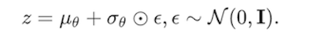
Now we transfer randomness to the random variable ∈ sampled from the Gaussian distribution. This makes the process differentiable since we could get the value ∈ during training. 💛
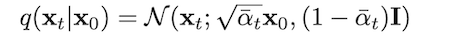
Property 2: Xt at any timestep can be represented by X0 and β
To obtain a noisy image Xt, we need to go through the Markov chain until we reach timestep t. Apparently, this process is very inefficient, especially in the DL training, which will have a bunch of input simultaneously.
Thanks to the reparameterization trick, we could now get the noisy image Xt by inputting the initial image X0 and the corresponding timestep t, based on the following formula:
(for the detail deducing process, I put it at the end of this section)
Finally, let's code the forward-nosing process base on Property 2 😄
The above shows two different versions of the Diffusion schedule, discrete and continuous. This implementation will focus on the former one.
For more information about continuous Diffusion schedules, I recommend reading the Keras example of the DDIM model.
Mathematical proof of Property 2
Our final target is to obtain the xT. By going through multiple Gaussian conditional probability q(xt|xt−1).
First, we redefine alpha and beta as below:
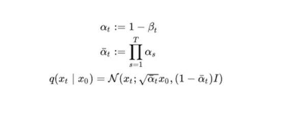
using the reparameterization trick we could rewrite q(xt|xt−1) as:
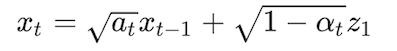
where z1 ~ N(0, I)
Expanding the xt we could get:
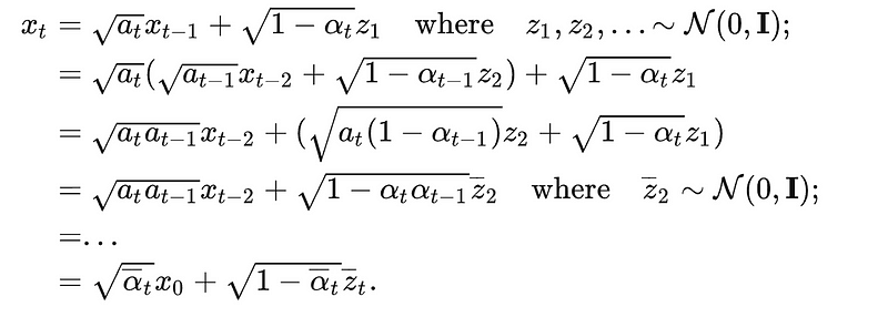
Since the merge of two Gaussians is also a Gaussians which is
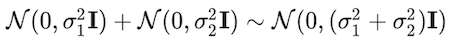
The merged standard deviation is

Finally, we could get the noisy image at any timestep using the result.
🥀 🥀 🥀 🥀 🥀🥀 🥀 🥀 🥀 🥀🥀 🥀 🥀 🥀 🥀🥀 🥀 🥀 🥀 🥀🥀 🥀 🥀🥀🥀🥀🥀🥀
Backward Denoising
If the forward process is the process of adding noise, then the backward process is to remove the noise.
If we could find the reverse distribution q(xt−1|xt), we can recreate the real image from Gaussian noise xT ~ N(0, I). Since q(xt|xt−1) is a Gaussian, if βt is small enough, q(xt−1|xt) will also be a Gaussian.
However, we couldn’t estimate the q easily since it needs to estimate the entire data distribution; thus, we will learn a model P to approximate this conditional probability. The distribution of p(xt−1|xt) is written as:
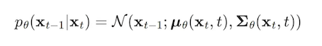
Our target is to obtain the initial state X0
DDPM
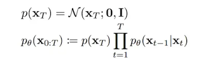
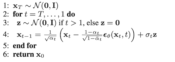
In the ddpm paper, the author defined the sampling process as:
The reverse distribution p(xt−1|xt) could be written as:
We use the U-net model to predict Є_θ with the input (xt, t), besides DDPM use untrain sigma_θ and believe sigma_θ (sigma_t in the above image ) approximate to βt
let's code this !!! ~~~ 😙
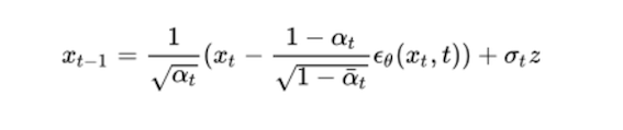
The above is the denoising process of DDPM. However, I am more prefer the DDIM denoising process, which is based on:
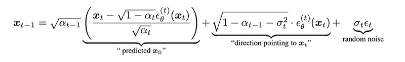
By setting the σ to 0, we could remove the randomness during sampling, reducing the inference time.
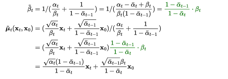
Mathematic behind the reverse process
Ok, it's time for some math ~~ 😢 😢
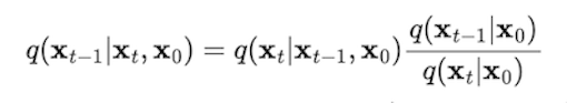
let us review the sampling process again. Our target is to get the reverse conditional probability q(xt−1|xt). To make it tractable, we first throw an X0 into it like this:
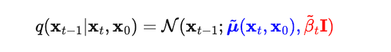
after applying Bayes’ rule, we have:
Now, all the q becomes forward, which means we could get the mean and variance of q based on Property 2 mentioned in the previous section.
Expanding the standard Gaussian density function of q, we could get:
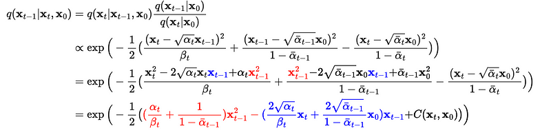
Keep expanding, we could get:
Finally, we only left X0 needs to be removed. Thanks to the reparameterization trick (Property 1), we could rewrite it as:
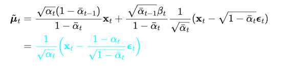
As shown above, the thing we need to have to process the denoising is Є_t which is equal to the input noise in the forward process, and the neural network can predict it. Yeah ~~ 😁 😁
Model Architecture and Training
In the diffusion model, we use a U-net structure to predict the noise Є_t by inputting image data X0 and timestep t.
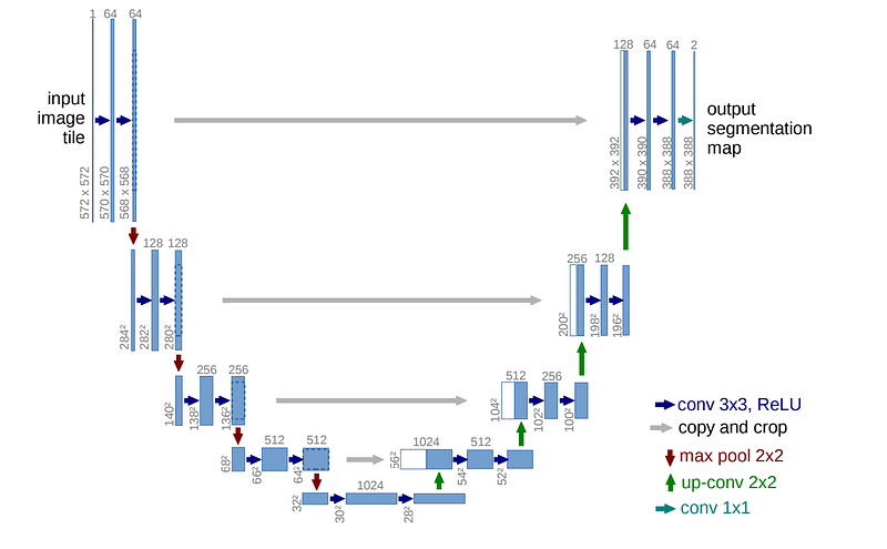
U-Net is a popular convolutional neural network (CNN) architecture, which was first developed for biomedical image segmentation. It is based on the convolutional layer to downsample and upsample the input image and adds skip connections between layers having the same resolution.
here is the link to the official paper of u-net
Let's write our diffusion model !! ~~~ 👐
Welcome to visit my GitHub. I have put the code on it ~~ 😸
U-net blocks
U-net model
For simplicity, I omit the attention layer, which could provide better global coherence. Besides, I use batch norm instead of group norm to reduce the amount of computation.
Training
We choose the mean squared error as the loss function for the model optimisation to calculate the loss between the noise (from the forward process) and the predicted noise (from the model).
But why can we use such a simple function as MSE to optimize the two distributions, p and q?
To answer this, I strongly recommend watching Ari Seff's youtube video and the Lil’Log. 🥀 🥀
Result
~~~~~~~~~~~~~~
Finally, I hope you enjoyed this article. I will write more articles related to AI, including explanations of their underlying principles and how to implement them
If that sounds interesting to you, feel free to follow me. 👏 😁
My Medium: link
My LinkedIn: link


