Stochastic Model for Dynamic Futures Basis Trading

Futures are standardized bilateral contracts of agreement to buy or sell an asset at a pre-determined price at a pre-specified time in the future. In the futures market, it is commonly observed that the futures prices may deviate from the spot price of the underlying asset. The differential between futures and spot prices, called the basis, can be positive or negative but are expected to converge to zero or near-zero at the expiration of the futures contract.

Basis Trading

Sometimes traders try to take advantage of the difference (called the basis) between the price of a futures contract and the spot price of contract’s underlying asset or index. This practice is commonly called basis trading.

Traders observe how the basis evolves over time and make trading decisions. If the basis is currently far from zero, then the trader may make a speculative bet that it will revert to zero in near future.

For each underlying asset, there are multiple futures with different maturities (ranging from 1 month to over a year). For each futures contract, there is one basis process. Therefore, when we consider all different spot assets and their associated futures, there are a high number of basis processes.

Moreover, these stochastic processes are clearly dependent. First, different underlying assets, such as silver and gold, can be correlated. Second, the futures contracts written on the same underlying asset are clearly driven by a common source of randomness, among other factors. For anyone trading futures — on the same underlying or different assets — it is crucial to understand the dependence structure among these processes.

Multidimensional Scaled Brownian Bridge

This motivates us to develop a novel model to capture the joint dynamics of stochastic basis from different underlying assets and different futures contracts. Once this model is built, one can apply it to dynamic futures trading.

The Multidimensional Scaled Brownian Bridge (MSBB) is a continuous-time stochastic model described by the following multidimensional stochastic differential equation (SDE):

where

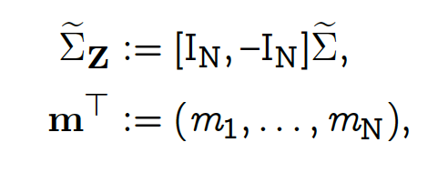
and W consists of Brownian motions.

In fact, Z is a N-dimensional process where each component is a 1-dimensional scaled Brownian bridge:

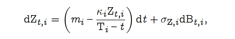
The stochastic differential equation for a 1-d scaled Brownian bridge. Note that the scaled Brownian bridges Zᵢ are correlated.

The SDE for the multidimensional scaled Brownian bridge has a unique solution

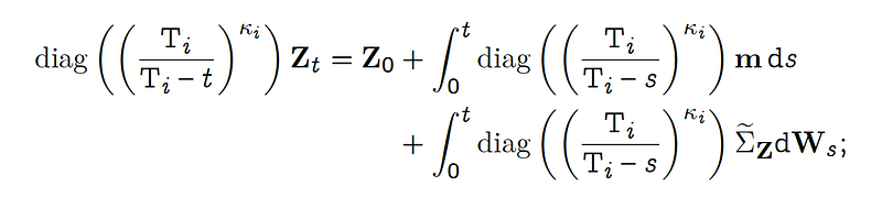
Here, we used the shorthand notation for the diagonal matrix: diag (aᵢ ) = diag(a₁ , . . . , aN).

The mean function of Z is given by

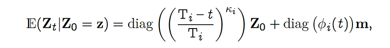
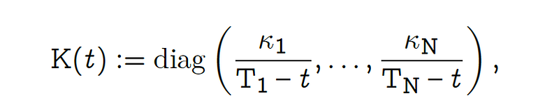
where

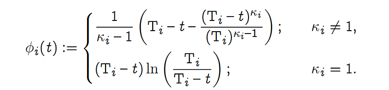
κᵢ is the scaling parameter.

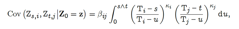
And the covariance function is

Path Behaviors

Figure 1 illustrates the simulated paths of Z, S, and F for two pairs of futures and underlying assets (i.e. N = 2). Here, each Z is the log basis (i.e. log(F/S)) for the corresponding asset and futures contract. The plots for (Zt,1) and (Zt,2) also show the 95% confidence intervals of the log-bases.

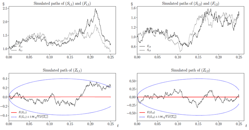
Figure 1: Simulated sample paths of S and F for two pairs of futures and spot (i.e. N = 2), and the corresponding 2-dimensional basis processes Z.

These plots showcase two characteristics of the log-bases. First, they are mean-reverting in that any deviation from their mean is corrected. Second, they partially converge to zero at the end of the trading horizon (T = 0.25) as evident by narrowing of the confidence intervals. Indeed, (Zt,1) and (Zt,2) are Brownian bridges that converge to zero at T₁ = 0.27 and T₂ = 0.254, respectively. This convergence is not realized since trading stops at T = 0.25 in this particular example.

Since, Zt|Z₀ is a multivariate normal random variable, this means that

has a chi-squared distribution with N degrees of freedom. This relationship is utilized for obtaining the 95% confidence regions of Zt represented by dashed blue ellipses. These plots also illustrate partial convergence of log-basis at the end of time horizon.

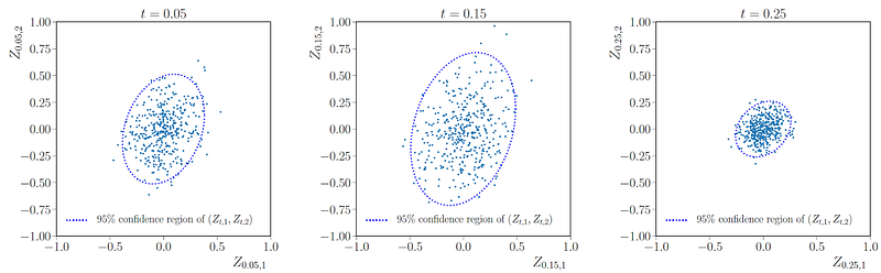
Simulated values of (Z₁, Z₂ ) based on 400 Simulated paths observed at three different times: t = 0.05 (left), t = 0.15 (middle), and t = 0.25(right). The dotted lines represent the border of the 95% confidence region for (Z₁, Z₂), conditional on Z₀ = (0,0).

Simulation

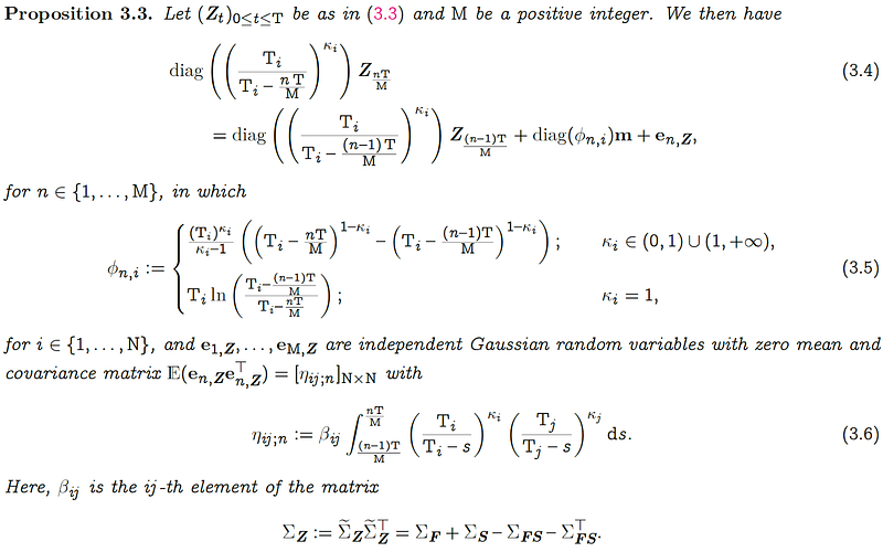
The SDE solution for the multidimensional scaled Brownian bridge actually lends itself to a simulation algorithm. We refer to the paper for details, but the main idea is to discretize the time horizon in M time steps, simulate independent Gaussian random variables, and put them in the right places as follows:

Source: Angoshtari and Leung (2020), available at https://arxiv.org/pdf/1910.04943.pdf

For any notations not explained herein, please refer to the papers below.

Takeaways

For trading systems that involve multiple futures and assets, it is imperative to properly capture the dependence among price processes. MSBB described herein is designed for modeling the joint dynamics among futures and their spot assets. Through the solution to the stochastic differential question, this model is straightforward to simulate. With simulated sample paths, one can test the performance of trading strategies.

References

B. Angoshtari and T. Leung, Optimal Trading of a Basket of Futures Contracts [pdf;link], Annals of Finance, 2020

B. Angoshtari and T. Leung, Optimal Dynamic Basis Trading [link;read online], Annals of Finance, Vol.15, Issue 3, pp. 307–335, 2019