Algo Trading

A Stopped Scaled Brownian Bridge Model for Basis Trading

Generating optimal positions from a new stochastic model

Futures are standardized bilateral contracts of agreement to buy or sell an asset at a pre-determined price at a pre-specified time in the future. The underlying assets can be physical commodities, market indexes, or financial instruments. The Chicago Mercantile Exchange (CME), which is the world’s largest futures exchange, averages well over 10 million futures contracts traded per day.

Sometimes traders try to take advantage of the difference (called the basis) between the price of a futures contract and the spot price of contract’s underlying asset or index. This practice is commonly called basis trading.

Traders observe how the basis evolves over time and make trading decisions. If the basis is currently far from zero, then the trader may make a speculative bet that it will revert to zero in near future.

Unlike stocks, the basis has a finite lifetime, and tends to go to zero as time approaches the expiration date of the futures contract. However, the basis doesn’t always completely vanish at expiry either. This non-convergence phenomenon was commonly observed in the grains markets. As a result, some cash-and-carry traders may choose to close their positions prior to maturity to limit risk exposure.

Traders must carefully account for these market phenomena in their trading strategies.

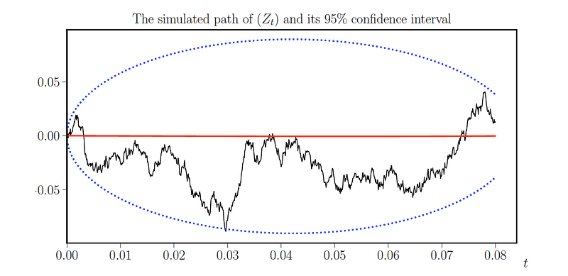
In order to capture these crucial features (i.e. tendency to zero towards the end but not perfect convergence), we model the stochastic basis by a scaled Brownian bridge that is stopped before its achieves convergence. The evolution of the basis is described by the stochastic differential equation

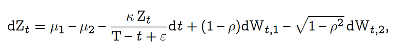
As we can see, the drift (the dt term) is negative when Z is positive, positive when Z is negative, and zero only when Z is zero. This creates a force of mean reversion driving the basis to zero, and the force is increasing rapidly (to infinity) as time t approaches T+ε (but the bridge is stopped at time T). The speed of the mean reversion is scaled by the parameter κ.

But this Brownian bridge is not pinned at zero as the futures matures. Instead, the bridge’s end point is random, representing the non-convergence between the futures and spot prices. The degree of non-convergence is controlled by the parameter ε > 0. If ε = 0, the futures price will converge exactly to the spot price.

In addition, there are two parameters μ₁ and μ₂, and two Brownian motions Wt,₁ and Wt,₂, which actually are inherited from the spot price and futures price processes. A detailed buildup of the model is here.

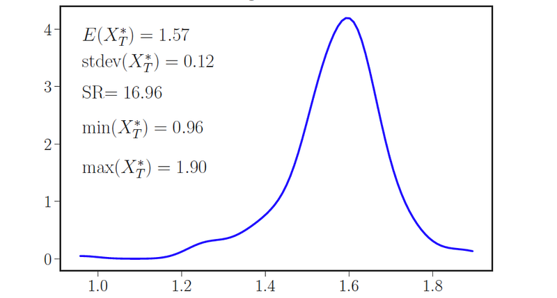
The optimal trading strategies are determined from a utility maximization problem under hyperbolic absolute risk aversion risk preferences. In our paper, we derive the exact conditions under which the equation admits a solution and solve the utility maximization explicitly. A series of numerical examples are provided to illustrate the optimal strategies and examine the effects of model parameters.

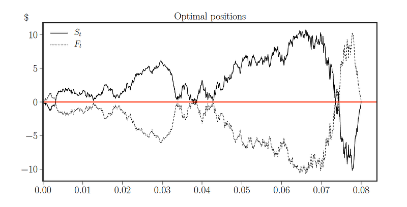
As it turns out, our approach automatically generates a dynamic long-short strategy to trade the basis over time. As such the position in the futures and underlying assets are of opposite signs (of different sizes).

Reference

Optimal Dynamic Basis Trading [link;read online], Annals of Finance, Vol.15, Issue 3, pp. 307–335, 2019 (w. Bahman Angoshtari)

Optimal Timing to Trade Along a Randomized Brownian Bridge [pdf;link], International Journal of Financial Studies, 6(3),75, pp.1–23, 2018 (with Jiao Li, Xin Li)

Google Scholar // Linkedin Page // Homepage

Learn more about University of Washington’s Computational Finance & Risk Management (CFRM) Program